Learn a Simplified Synthesis of Financial Options Pricing

Financial options (the right to purchase (“call“) or sell (“put“) stock (or other assets)) at a fixed price at a future date have been around for a long time. They are attractive for the option buyer since his/her total risk is the premium (price) paid for the option, as contrasted with futures contracts which are obligations to buy a stock or commodity at a future date.  However, until recently, financial options pricing presented great difficulties and controversy: how do you put a fair price on an asset deliverable at a future date, sometimes years ahead?  Then in 1973 Drs. F. Black, M. Scholes, and  R.C. Merton published a model for options pricing based essentially on Gaussian (random-walk) probability.

The following is the famed Black-Scholes equation for determining the “fair” price of a call or put option.

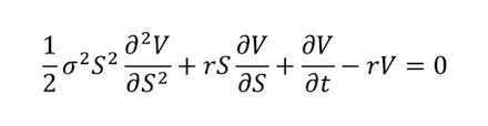
Some of the  involved math may be gleaned from the following excerpt of its derivation:

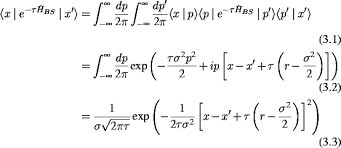
And finally the formula itself:

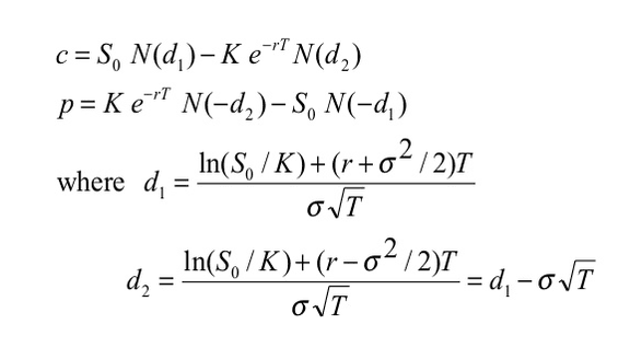
where c is the cost of a call option and p the cost of a put option. I  won’t discuss the remaining parameters since we won’t be using this model directly.

As a purely theoretical inquiry, what mathematics lies behind the Black-Scholes formula?  I have long wondered and marveled at its complexity.  After all, it’s supposedly based on Gaussian probability aka random walk. Certainly, the formula does not lend itself to a ready understanding of what lies behind rational options pricing.  Is there a simpler, more intuitive approach yielding the same quantitative results coupled with deeper insight into options pricing rationale?  I propose one herewith.

I am assuming a very basic familiarity with put and call options  All you need to know is the spot price, strike price, duration, and (annualized) volatility.   By “volatility” the financier specifically means the standard deviation of the spread of underlying stock prices over a 1 year period.    (Interest rate is usually another input and will be touched on later.)

At this point, I need to mention that the sole option price that has to be determined is the call price.  The put price for the same input parameters is immediately derivable from the so-called put-call parity rule, which is just (call price) – (put price) = (spot price) – (strike price).  So I will limit myself to call options.

Another thing to mention is that the below applies strictly speaking to so-called European options only; however, there is very little difference in price between these and so-called American options, usually well below 1%.  An online Black-Scholes options price calculator makes this clear.  Another easy-to-use Black-Scholes calculator for call options is at mystockoptions.com.

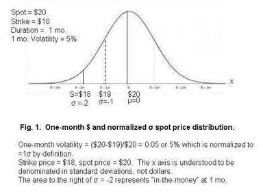
Let us go by way of an example.  Assume the spot price is $20 and the strike price $18; also that the volatility is $1 or 1/20 = 5% on a one-month basis (which is $\frac 1 {\sqrt12}$of  the annualized volatility).  This means the mean is $20 and the standard deviation for 1 month of data is $1.    See fig. 1.

We will now develop the necessary data to determine the price of a 3-month call option. At three months the strike price will represent less than 2  std. deviations since the price structure will now be “spread out” by a factor of  $\sqrt 3$.  The 3-month distribution will then look like fig.2.

 

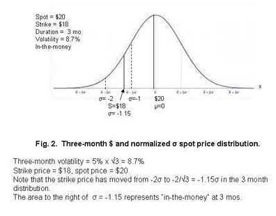
Notably, the $18 strike price now represents not -2σ but -2/$\sqrt 3$ = -1.15σ.  So the area under the probability density function to the right of that value represents the probability that the price will be > strike price after 3 months in which case the option has value.

But that is not the whole story.  The other question is “ok, but what will be the average value assuming the option does have value?  Clearly, we want the average of the x-axis to the right of the strike price, i.e. x adjusted such that at x = -1.15 the contract value is 0.

So let’s do some probability.  Let f(x) be the probability density function and F(x) the cumulative function, i.e. the area from -$\infty$ to x.  The entire area = 1 so $F(\infty)$ = 1.  Then the average value of x such that F(-1.15) = 0 will be, noting that F(-x) = F(1-x),

$$ \bar x = \int_{-1.15}^{\infty} (x – (-1.15)) f(x) \, dx$$

$$ = 1.15\int_{-1.15}^{\infty} f(x) \, dx + \int_{-1.15}^{ \infty} x f(x) \, dx.$$

So what to do with the last integral?  No tables, nothing!  But we are saved by a very felicitous relation which is x f(x) = – f ‘(x)

so now we get

$$ \bar x = 1.15\int_{-1.15}^{\infty} f(x) \, dx  \text{} ~  –  \int_{-1.15}^{\infty} f ‘(x) \, dx.$$    or

$$ \bar x = 1.15F(1.15) – [(f(\infty) – f(1.15)] $$

= 1.15F(1.15) + f(1.15)

$\bar x$ = 0.875 + 0.206 = 1.212

Finally we multiply by the dollar value corresponding to $\sqrt 3$ to get cost c = ($1.73)(1.212) = $2.09.

Comparing this with the Black-Scholes calculator with the substitution $\sigma_{1 yr} = \sqrt{(12/3)}\sigma_{3 mos.}$ to  annualize the volatility we get $2.09.  Exactly the same price as ours.

Let’s proceed with an out-of-the-money case, i.e. when the strike price is above the spot price.  For this I chose as follows:

spot = $20

strike = $25

1 month volatility = $2 = 1σ

duration = 3 mos.  See fig. 3.  This is very much an out-of-the-money option, obviously.

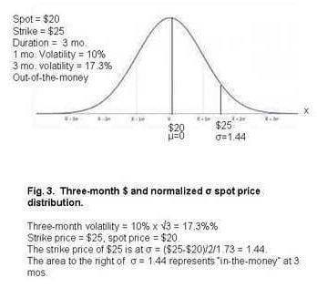
The approach is the same:  the integration to obtain average x again starts at the σ equivalent of the strike price which will be ($25-$20)/2.5/1.73 = 1.44.  So to find the average x starting at 1.44 we need

$$\int_{1.44}^{\infty} (x – 1.44) f(x) \, dx$$ = f(1.44) – 1.44(1 – F(1.44)) = .142 – 1.44(0.075) = 0.034 x ($2 x 1.73) = $0.11 vs. $0.19 for the Black-Scholes model. Presumably, roundoff error accounts for the difference.

In general the price of any call option will be

$$ c = \left( \frac $ \sigma \right)  \int_{\sigma_{strike}}^{\infty} (x – \sigma_{strike}) f(x) \, dx $$

with $\sigma = \sqrt{n/\sigma_v}$ , n the duration in years and $\sigma_v$ = (annualized) volatility.

I further tested the model with spot = strike = $20, and got $0.69 which agreed exactly with the Black-Scholes calculation.

The prevailing interest rate should figure in these computations.  It’s easily taken care of by simply accounting for the “present value” of the payout.  The same can be said for inflation, which at this date (Aug. 2018) is actually greater than the “safe” short-term interest rate.

I’ve appended an excel file $^{(1)}$ that enables these computations for any combination of spot, strike, duration, and volatility.  (The program delineates between in-the-money and out-of-the-money cases).

Should this model be used for options pricing rather than the Black-Scholes?  No.  The latter has been assiduously nurtured over the decades and can allegedly handle more input parameters. Online calculators facilitate its application. The point of this investigation is rather to gain insight into options pricing mathematics by formulating a much-simplified basis of evaluating options, based on Gaussian variation like the Black-Scholes model, yet yielding the same results as the latter model in a much more understandable way.

Then too, how valuable is any model based on random theory really?  The infamous collapse of the hedge fund Long-Term Capital Management in 1999, in which Dr. Scholes was a participating investor, answers that question nicely, as does the 2008 general financial collapse.  I recommend reading N. Taleb’s The Black Swan for casting further doubt on the predictability of any stochastic future pricing models.  He shows that there can be and usually are severe bumps on those cherished smooth Gaussian curves!

Resources:

(1) Copy of rude man call option calculator

Additional (duplicate) ppt slides for the three embedded figures.  These are of better quality than the embodied ones:   blk-sch.ppt