
Answering Mermin’s Challenge with the Relativity Principle
Note: This Insight was previously titled, “Answering Mermin’s Challenge with Wilczek’s Challenge.” While that version of this Insight did not involve any particular interpretation of quantum mechanics, it did involve the block universe interpretation of special relativity. I have updated this Insight to remove the block universe interpretation, so that it now answers Mermin’s challenge in “principle” fashion alone, as in this Insight.
Nearly four decades ago, Mermin revealed the conundrum of quantum entanglement for a general audience [1] using his “simple device,” which I will refer to as the “Mermin device” (Figure 1). To understand the conundrum of the device required no knowledge of physics, just some simple probability theory, which made the presentation all the more remarkable. Concerning this paper Feynman wrote to Mermin, “One of the most beautiful papers in physics that I know of is yours in the American Journal of Physics” [2, p. 366-7]. In subsequent publications, he “revisited” [3] and “refined” [4] the mystery of quantum entanglement with similarly simple devices. In this Insight, I will focus on the original Mermin device as it relates to the mystery of entanglement via the Bell spin states.
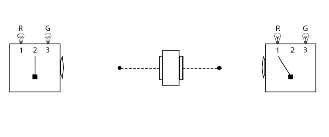
Figure 1. The Mermin Device
The Mermin device functions according to two facts that are seemingly contradictory, thus the mystery. Mermin simply supplies these facts and shows the contradiction, which the “general reader” can easily understand. He then challenges the “physicist reader” to resolve the mystery in an equally accessible fashion for the “general reader.” Here is how the Mermin device works.
The Mermin device is based on the measurement of spin angular momentum (Figure 2). The spin measurements are carried out with Stern-Gerlach (SG) magnets and detectors (Figure 3). The Mermin device contains a source (middle box in Figure 1) that emits a pair of spin-entangled particles towards two detectors (boxes on the left and right in Figure 1) in each trial of the experiment. The settings (1, 2, or 3) on the left and right detectors are controlled randomly by Alice and Bob, respectively, and each measurement at each detector produces either a result of R or G. The following two facts obtain:
- When Alice and Bob’s settings are the same in a given trial (“case (a)”), their outcomes are always the same, ##\frac{1}{2}## of the time RR (Alice’s outcome is R and Bob’s outcome is R) and ##\frac{1}{2}## of the time GG (Alice’s outcome is G and Bob’s outcome is G).
- When Alice and Bob’s settings are different (“case (b)”), the outcomes are the same ##\frac{1}{4}## of the time, ##\frac{1}{8}## RR and ##\frac{1}{8}## GG.
The two possible Mermin device outcomes R and G represent two possible spin measurement outcomes “up” and “down,” respectively (Figure 2), and the three possible Mermin device settings represent three different orientations of the SG magnets (Figures 3 & 4).
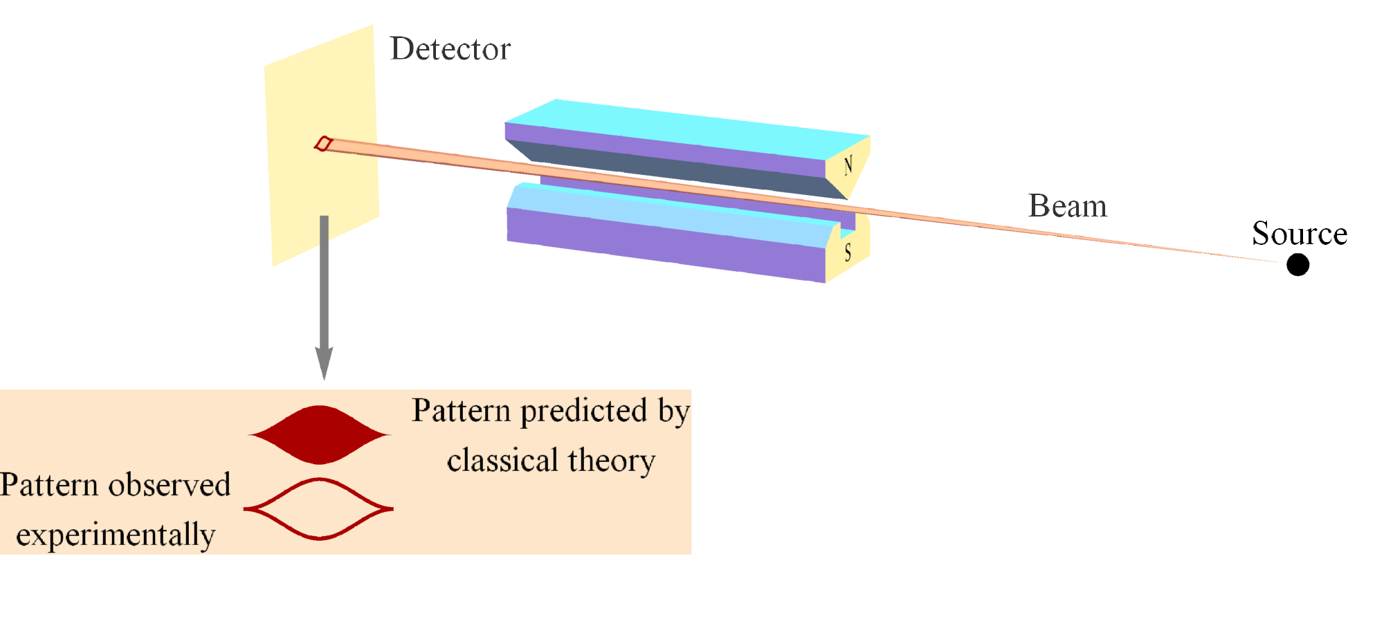
Figure 2. A pair of Stern-Gerlach (SG) magnets showing the two possible outcomes, up (##+\frac{\hbar}{2}##) and down (##-\frac{\hbar}{2}##) or ##+1## and ##-1##, for short. The important point to note here is that the classical analysis predicts all possible deflections, not just the two that are observed. This difference uniquely distinguishes the quantum joint distribution from the classical joint distribution for spin entangled pairs [5].

Figure 3. Alice and Bob making spin measurements on a pair of spin-entangled particles with their SG magnets and detectors. In this particular case, the plane of conserved spin angular momentum is the xz plane.
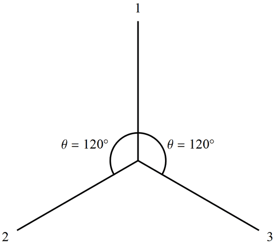
Figure 4. Three orientations of SG magnets in the plane of symmetry for Alice and Bob’s spin measurements corresponding to the three settings on the Mermin device.
Mermin writes, “Why do the detectors always flash the same colors when the switches are in the same positions? Since the two detectors are unconnected there is no way for one to ‘know’ that the switch on the other is set in the same position as its own.” This leads him to introduce “instruction sets” to account for the behavior of the device when the detectors have the same settings. He writes, “It cannot be proved that there is no other way, but I challenge the reader to suggest any.” Now look at all trials when Alice’s particle has instruction set RRG and Bob’s has instruction set RRG, for example.
That means Alice and Bob’s outcomes in setting 1 will both be R, in setting 2 they will both be R, and in setting 3 they will both be G. That is, the particles will produce an RR result when Alice and Bob both choose setting 1 (referred to as “11”), an RR result when both choose setting 2 (referred to as “22”), and a GG result when both choose setting 3 (referred to as “33”). That is how instruction sets guarantee Fact 1. For different settings, Alice and Bob will obtain the same outcomes when Alice chooses setting 1 and Bob chooses setting 2 (referred to as “12”), which gives an RR outcome. And, they will obtain the same outcomes when Alice chooses setting 2 and Bob chooses setting 1 (referred to as “21”), which also gives an RR outcome. That means we have the same outcomes for different settings in 2 of the 6 possible case (b) situations, i.e., in ##\frac{1}{3}## of case (b) trials for this instruction set. This ##\frac{1}{3}## ratio holds for any instruction set with two R(G) and one G(R).
The only other possible instruction sets are RRR or GGG where Alice and Bob’s outcomes will agree in ##\frac{9}{9}## of all trials. Thus, the “Bell inequality” for the Mermin device says that instruction sets must produce the same outcomes in more than ##\frac{1}{3}## of all case (b) trials. But, Fact 2 for the Mermin device says you only get the same outcomes in ##\frac{1}{4}## of all case (b) trials, thereby violating the Bell inequality. Thus, the conundrum of Mermin’s device is that the instruction sets needed for Fact 1 fail to yield the proper outcomes for Fact 2.
Concerning his device Mermin wrote, “Although this device has not been built, there is no reason in principle why it could not be, and probably no insurmountable practical difficulties.” Sure enough, the experimental confirmation of the violation of Bell’s inequality per quantum entanglement is so common that it can now be carried out in the undergraduate physics laboratory [6]. Thus, there is no disputing that the conundrum of the Mermin device has been experimentally well verified, vindicating its prediction by quantum mechanics.
While the conundrum of the Mermin device is now a well-established fact, Mermin’s “challenging exercise to the physicist reader to translate the elementary quantum-mechanical reconciliation of cases (a) and (b) into terms meaningful to a general reader struggling with the dilemma raised by the device” arguably remains unanswered. To answer this challenge, it is generally acknowledged that one needs a compelling causal mechanism or a compelling physical principle by which the conundrum of the Mermin device is resolved. Such a model needs to do more than the “Copenhagen interpretation” [7], which Mermin characterized as “shut up and calculate” [8]. In other words, while the formalism of quantum mechanics accurately predicts the conundrum, quantum mechanics does not provide a model of physical reality or underlying physical principle to resolve the conundrum. While there are many interpretations of quantum mechanics, even one published by Mermin [9], there is no consensus among physicists on any given interpretation.
Rather than offer yet another uncompelling interpretation of quantum mechanics, I will share and expand on an underlying physical principle [10,11] that explains the quantum correlations responsible for the conundrum of the Mermin device. In other words, I will provide a “principle account” of quantum entanglement. Here I’m making specific reference to Einstein’s notion of a “principle theory” as explained in this Insight. While this explanation, conservation per no preferred reference frame (NPRF), may not be “in terms meaningful to a general reader,” it is pretty close. That is, all one needs to appreciate the explanation is a course in introductory physics, which probably represents the “general reader” interested in this topic.
That quantum mechanics accurately predicts the observed phenomenon without spelling out any means a la “instruction sets” for how it works prompted Smolin to write [12, p. xvii]:
I hope to convince you that the conceptual problems and raging disagreements that have bedeviled quantum mechanics since its inception are unsolved and unsolvable, for the simple reason that the theory is wrong. It is highly successful, but incomplete.
Of course, this is precisely the complaint leveled by Einstein, Podolsky and Rosen (EPR) in their famous 1935 paper [13], “Can Quantum-Mechanical Description of Physical Reality Be Considered Complete?” Contrary to this belief, I will show that quantum mechanics is actually as complete as possible, given Einstein’s own relativity principle (NPRF). Indeed, Einstein missed a chance to rid us of his “spooky actions at a distance.” All he would have had to do is extend his relativity principle to include the measurement of Planck’s constant h, just as he had done by extending the relativity principle from mechanics to include the measurement of the speed of light c per electromagnetism.
That is, the relativity principle (NPRF) entails the light postulate of special relativity, i.e., that everyone measure the same speed of light c, regardless of their motion relative to the source. If there was only one reference frame for a source in which the speed of light equalled the prediction from Maxwell’s equations (##c = \frac{1}{\sqrt{\mu_o\epsilon_o}}##), then that would certainly constitute a preferred reference frame. The light postulate then leads to time dilation, length contraction, and the relativity of simultaneity per the Lorentz transformations of special relativity. Indeed, this is the way special relativity is introduced by Serway & Jewett [14] and Knight [15] for introductory physics students. Let me show you how further extending NPRF to the measurement of Planck’s constant h leads to quantum entanglement per the qubit Hilbert space structure (probability structure) of quantum mechanics.
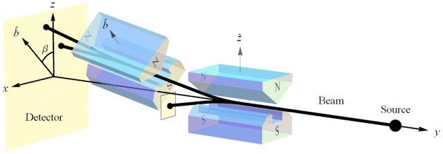
Figure 5. In this set up, the first SG magnets (oriented at ##\hat{z}##) are being used to produce an initial state ##|\psi\rangle = |u\rangle## for measurement by the second SG magnets (oriented at ##\hat{b}##).
As Weinberg points out [16], measuring an electron’s spin via SG magnets constitutes the measurement of “a universal constant of nature, Planck’s constant” (Figure 2). So if NPRF applies equally here, then everyone must measure the same value for Planck’s constant h, regardless of their SG magnet orientations relative to the source, which like the light postulate is an “empirically discovered” fact. By “relative to the source,” I might mean relative “to the vertical in the plane perpendicular to the line of flight of the particles” [1], ##\hat{z}## in Figure 5 for example. Here the possible spin outcomes ##\pm\frac{\hbar}{2}## represent a fundamental (indivisible) unit of information per Dakic & Brukner’s first axiom in their information-theoretic reconstruction of quantum theory [17], “An elementary system has the information carrying capacity of at most one bit.” Thus, different SG magnet orientations relative to the source constitute different “reference frames” in quantum mechanics just as different velocities relative to the source constitute different “reference frames” in special relativity.
To make the analogy more explicit, one could have employed NPRF to predict the light postulate as soon as Maxwell showed electromagnetic radiation propagates at ##c = \frac{1}{\sqrt{\mu_o\epsilon_o}}##. All they would have had to do is extend the relativity principle from mechanics to electromagnetism. However, given the understanding of waves at the time, everyone rather began searching for a propagation medium, i.e., the luminiferous ether. Likewise, one could have employed NPRF to predict spin angular momentum as soon as Planck published his wavelength distribution function for blackbody radiation. All they would have had to do is extend the relativity principle from mechanics and electromagnetism to quantum physics. However, given the understanding of angular momentum and magnetic moments at the time, Stern & Gerlach rather expected to see their silver atoms deflected in a continuum distribution after passing through their magnets (Figure 2). In other words, they discovered spin angular momentum when they were simply looking for angular momentum. But, had they noticed that their measurement constituted a measurement of Planck’s constant (with its dimension of angular momentum), they could have employed NPRF to predict the spin outcome with its qubit Hilbert space structure (Figures 2 & 5) and its ineluctably probabilistic nature, as I will now explain.
If we create a preparation state oriented along the positive ##z## axis as in Figure 5, i.e., ##|\psi\rangle = |u\rangle## in the Dirac notation [18], our spin angular momentum is ##\vec{S} = +1\hat{z}## (in units of ##\frac{\hbar}{2} = 1##). Now proceed to make a measurement with the SG magnets oriented at ##\hat{b}## making an angle ##\beta## with respect to ##\hat{z}## (Figure 5). According to classical physics, we expect to measure ##\vec{S}\cdot\hat{b} = \cos{(\beta)}## (Figure 6), but we cannot measure anything other than ##\pm 1## due to NPRF (contra the prediction by classical physics), so we see that NPRF answers Wheeler’s “Really Big Question,” “Why the quantum?” in “one clear, simple sentence” to convey “the central point and its necessity in the construction of the world” [19,20].
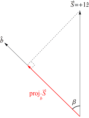
Figure 6. The spin angular momentum of Bob’s particle ##\vec{S}## projected along his measurement direction ##\hat{b}##. This does not happen with spin angular momentum due to NPRF.
As a consequence, we can only recover ##\cos{(\beta)}## on average (Figure 7), i.e., NPRF dictates “average-only” projection
\begin{equation}
(+1) P(+1 \mid \beta) + (-1) P(-1 \mid \beta) = \cos (\beta) \label{AvgProjection}
\end{equation}
Solving simultaneously with our normalization condition ##P(+1 \mid \beta) + P(-1 \mid \beta) = 1##, we find that
\begin{equation}
P(+1 \mid \beta) = \mbox{cos}^2 \left(\frac{\beta}{2} \right) \label{UPprobability}
\end{equation}
and
\begin{equation}
P(-1 \mid \beta) = \mbox{sin}^2 \left(\frac{\beta}{2} \right) \label{DOWNprobability}
\end{equation}
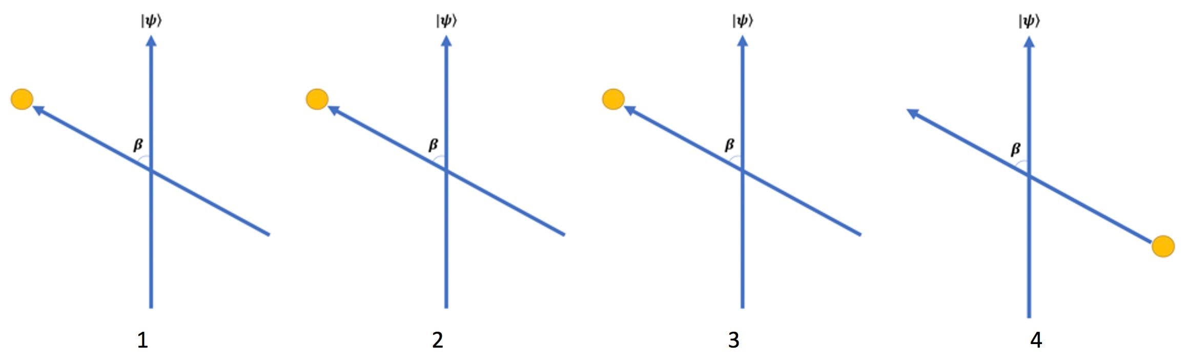
Figure 7. An ensemble of 4 SG measurement trials with ##\beta = 60^{\circ}##. The tilted blue arrow depicts an SG measurement orientation and the vertical arrow represents our preparation state ##|\psi\rangle = |u\rangle## (Figure 5). The yellow dots represent the two possible measurement outcomes for each trial, up (located at arrow tip) or down (located at bottom of arrow). The expected projection result of ##\cos{(\beta)}## cannot be realized because the measurement outcomes are binary (quantum) with values of ##+1## (up) or ##-1## (down) per NPRF. Thus, we have “average-only” projection for all 4 trials (three up outcomes and one down outcome for ##\beta = 60^\circ## average to ##\cos{(60^\circ)}=\frac{1}{2}##).
This explains the ineluctably probabilistic nature of QM, as pointed out by Mermin [21]:
Quantum mechanics is, after all, the first physical theory in which probability is explicitly not a way of dealing with ignorance of the precise values of existing quantities.
That is, quantum mechanics is as complete as possible, given the relativity principle. Of course, these “average-only” results due to “no fractional outcomes per NPRF” hold precisely for the qubit Hilbert space structure of quantum mechanics [11]. Thus, we see that NPRF provides a principle explanation of the kinematic/probability structure of quantum mechanics, just as it provides a principle explanation of the kinematic/Minkowski spacetime structure of special relativity. In fact, this follows from Information Invariance & Continuity at the basis of axiomatic reconstructions of QM per information-theoretic principles (see No Preferred Reference Frame at the Foundation of Quantum Mechanics). Now let’s expand this idea to the situation when we have two entangled particles, as in the Mermin device. The concept we need to understand now is the “correlation function.”
The correlation function between two outcomes over many trials is the average of the two values multiplied together. In this case, there are only two possible outcomes for any setting, +1 (up or R) or –1 (down or G), so the largest average possible is +1 (total correlation, RR or GG, as when the settings are the same) and the smallest average possible is –1 (total anti-correlation, RG or GR). One way to write the equation for the correlation function is
\begin{equation}\langle \alpha,\beta \rangle = \sum (i \cdot j) \cdot p(i,j \mid \alpha,\beta) \label{average}\end{equation}
where ##p(i,j \mid \alpha,\beta)## is the probability that Alice measures ##i## and Bob measures ##j## when Alice’s SG magnet is at angle ##\alpha## and Bob’s SG magnet is at angle ##\beta##, and ##(i \cdot j)## is just the product of the outcomes ##i## and ##j##. The correlation function for instruction sets for case (a) is the same as that of the Mermin device for case (a), i.e., they’re both 1. Thus, we must explore the difference between the correlation function for instruction sets and the Mermin device for case (b).
To get the correlation function for instruction sets for different settings, we need the probabilities of measuring the same outcomes and different outcomes for case (b), so we can use Eq. (\ref{average}). We saw that when we had two R(G) and one G(R), the probability of getting the same outcomes for different settings was ##\frac{1}{3}## (this would break down to ##\frac{1}{6}## for each of RR and GG overall). Thus, the probability of getting different outcomes would be ##\frac{2}{3}## for these types of instruction sets (##\frac{1}{3}## for each of RG and GR). That gives a correlation function of
\begin{equation}\langle \alpha,\beta \rangle = \left(+1\right)\left(+1\right)\left(\frac{1}{6}\right) + \left(-1\right)\left(-1\right)\left(\frac{1}{6}\right) + \left(+1\right)\left(-1\right)\left(\frac{2}{6}\right) + \left(-1\right)\left(+1\right)\left(\frac{2}{6}\right)= -\frac{1}{3}
\end{equation}
For the other type of instruction sets, RRR and GGG, we would have a correlation function of ##+1## for different settings, so overall the correlation function for instruction sets for different settings has to be larger than ##-\frac{1}{3}##. In fact, if all eight possible instruction sets are produced with equal frequency, then for any given pair of case (b) settings, e.g., 12 or 13 or 23, you will obtain RR, GG, RG, and GR in equal numbers giving a correlation function of zero. That means the results are uncorrelated as one would expect given that all possible instruction sets are produced randomly, i.e., with equal frequency. From this we would typically infer that there is nothing that needs to be explained.
Fact 2 for the Mermin device says the probability of getting the same results (RR or GG) for different settings is ##\frac{1}{4}## (##\frac{1}{8}## for each of RR and GG). Thus, the probability of getting different outcomes for case (b) must be ##\frac{3}{4}## (##\frac{3}{8}## for each of RG and GR). That gives a correlation function of
\begin{equation}\langle \alpha,\beta \rangle = \left(+1\right)\left(+1\right)\left(\frac{1}{8}\right) + \left(-1\right)\left(-1\right)\left(\frac{1}{8}\right) + \left(+1\right)\left(-1\right)\left(\frac{3}{8}\right) + \left(-1\right)\left(+1\right)\left(\frac{3}{8}\right)= -\frac{1}{2}
\end{equation}
That means the Mermin device is more strongly anti-correlated for different settings than instruction sets. Indeed, if all possible instruction sets are produced with equal frequency, the Mermin device evidences something to explain (anti-correlated results) where instruction sets suggest there is nothing to explain (uncorrelated results). Thus, quantum mechanics predicts and we observe anti-correlated outcomes for different settings in need of explanation while its classical counterpart suggests there is nothing in need of explanation at all. Mermin’s challenge then amounts to explaining why that is true for the “general reader.”
At this point read my Insight Exploring Bell States and Conservation of Spin Angular Momentum.
Now you understand how the correlation function for the Bell spin states results from “average-only” conservation (as a mathematical fact, Figure 8) resulting from the fact that Alice and Bob both always measure ##\pm 1 \left(\frac{\hbar}{2}\right)## (quantum), never a fraction of that amount (classical), as shown in Figure 2 (empirical fact).
There are two important points to be made here. First, NPRF is just the statement of an “empirically discovered” fact, i.e., Alice and Bob both always measure ##\pm 1##. Second, it is simply a mathematical fact that the “average-only” conservation yields the quantum correlation functions. In other words, to paraphrase Einstein, “we have an empirically discovered principle that gives rise to mathematically formulated criteria which the separate processes or the theoretical representations of them have to satisfy.” That is why this principle account of quantum entanglement provides “logical perfection and security of the foundations.” Thus, we see how quantum entanglement follows from NPRF applied to the measurement of h in precisely the same manner that time dilation and length contraction follow from NPRF applied to the measurement of c. And, just like in special relativity, Bob could partition the data according to his equivalence relation (per his reference frame) and claim that it is Alice who must average her results (obtained in her reference frame) to conserve spin angular momentum (Figure 9).
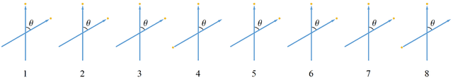
Figure 8. An ensemble of 8 experimental trials for the Bell spin states showing Bob’s outcomes corresponding to Alice‘s ##+1## outcomes when ##\theta = 60^\circ##. Angular momentum is not conserved in any given trial, because there are two different measurements being made, i.e., outcomes are in two different reference frames, but it is conserved on average for all 8 trials (six up outcomes and two down outcomes average to ##\cos{60^\circ}=\frac{1}{2}##). It is impossible for angular momentum to be conserved explicitly in each trial since the measurement outcomes are binary (quantum) with values of ##+1## (up) or ##-1## (down) per NPRF. The conservation principle at work here assumes Alice and Bob’s measured values of spin angular momentum are not mere components of some hidden angular momentum with variable magnitude. That is, the measured values of angular momentum are the angular momenta contributing to this conservation, as I explained in my Insight Bell States and Conservation of Spin Angular Momentum.
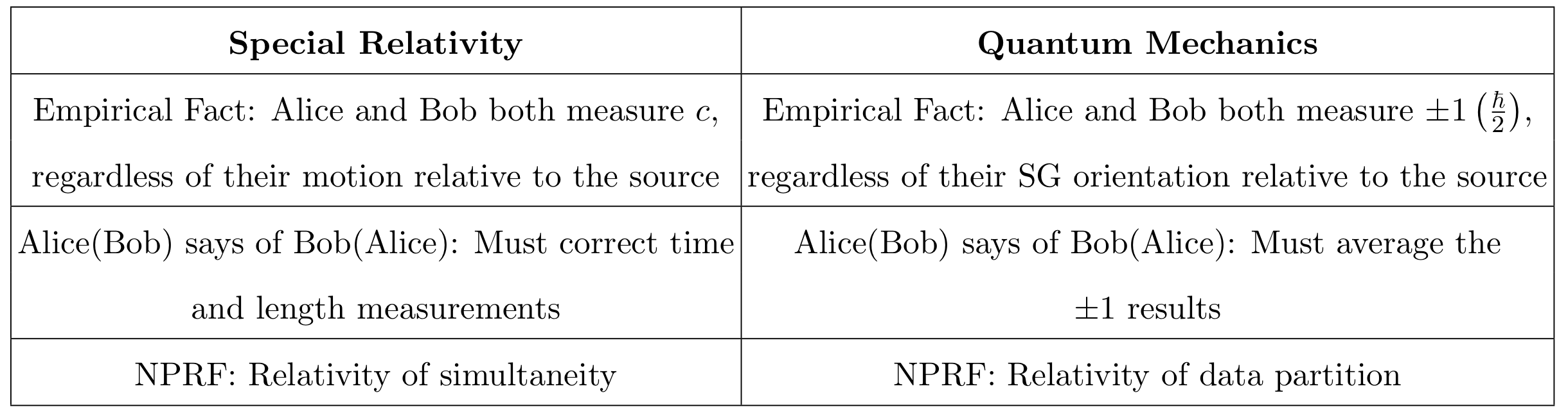
Figure 9. Comparing special relativity with quantum mechanics according to no preferred reference frame (NPRF).
Of course, all of this does not provide any relief for those who still require explanation via “constructive efforts.” As Lorentz complained [22]:
Einstein simply postulates what we have deduced, with some difficulty and not altogether satisfactorily, from the fundamental equations of the electromagnetic field.
And, Albert Michelson said [23]:
It must be admitted, these experiments are not sufficient to justify the hypothesis of an ether. But then, how can the negative result be explained?
In other words, neither was convinced that NPRF was sufficient to explain time dilation and length contraction. Apparently for them, such a principle must be accounted for by some causal mechanism, e.g., the luminiferous ether. Likewise, if one requires “constructive efforts” to account for “conservation per NPRF” responsible for “average-only” conservation, then they will certainly want to continue the search for a causal mechanism responsible for quantum entanglement.
But after 115 years, physicists have largely abandoned theories of the luminiferous ether, having grown comfortable with the longstanding and empirically sound light postulate based on NPRF. Even Lorentz seemed to acknowledge the value of this principle explanation when he wrote [22]:
By doing so, [Einstein] may certainly take credit for making us see in the negative result of experiments like those of Michelson, Rayleigh, and Brace, not a fortuitous compensation of opposing effects but the manifestation of a general and fundamental principle.
Therefore, 85 years after publication of the EPR paper, perhaps we should consider the possibility that quantum entanglement will likewise ultimately yield to principle explanation. After all, we now know that our time-honored relativity principle is precisely the principle that resolves the mystery of “spooky actions at a distance.” As John Bell said in 1993 [24, p. 85]:
I think the problems and puzzles we are dealing with here will be cleared up, and … our descendants will look back on us with the same kind of superiority as we now are tempted to feel when we look at people in the late nineteenth century who worried about the ether. And Michelson-Morley .., the puzzles seemed insoluble to them. And came Einstein in nineteen five, and now every schoolboy learns it and feels .. superior to those old guys. Now, it’s my feeling that all this action at a distance and no action at a distance business will go the same way. But someone will come up with the answer, with a reasonable way of looking at these things. If we are lucky it will be to some big new development like the theory of relativity.
Perhaps causal accounts of quantum entanglement are destined to share the same fate as theories of the luminiferous ether. Regardless, we have certainly answered Mermin’s challenge, since conservation per NPRF is very accessible to the “general reader.”
References
- Mermin, N.D.: Bringing home the atomic world: Quantum mysteries for anybody. American Journal of Physics 49, 940-943 (1981).
- Feynman, M.: Perfectly Reasonable Deviations from the Beaten Track. Basic Books, New York (2005).
- Mermin, N.D.: Quantum mysteries revisited. American Journal of Physics 58, 731-734 (Aug 1990).
- Mermin, N.D.: Quantum mysteries refined. American Journal of Physics 62, 880-887 (Aug 1994).
- Garg, A., and Mermin, N.D.: Bell Inequalities with a Range of Violation that Does Not Diminish as the Spin Becomes Arbitrarily Large. Physical Review Letters 49(13), 901–904 (1982).
- Dehlinger, D., and Mitchell, M.W.: Entangled photons, nonlocality, and Bell inequalities in the undergraduate laboratory. American Journal of Physics 70(9), 903–910 (2002).
- Becker, A.: What is Real? The Unfinished Quest for the Meaning of Quantum Physics. Basic Books, New York (2018).
- Mermin, N.D.: Could Feynman Have Said This? Physics Today 57(5), 10 (Apr 2004).
- Mermin, N.D.: What is quantum mechanics trying to tell us? American Journal of Physics 66(9), 753-767 (1998).
- Stuckey, W.M., Silberstein, M., and McDevitt, T., and Le, T.D.: Answering Mermin’s challenge with conservation per no preferred reference frame. Scientific Reports 10, 15771 (2020).
- Silberstein, M., Stuckey, W.M., and McDevitt, T.: Beyond Causal Explanation: Einstein’s Principle Not Reichenbach’s. Entropy 23(1), 114 (2021).
- Smolin, L.: Einstein’s Unfinished Revolution: The Search for What Lies Beyond the Quantum. Penguin Press, New York (2019).
- Einstein, A., Podolsky, B., and Rosen, N.: Can Quantum-Mechanical Description of Physical Reality Be Considered Complete? Physical Review 47(10), 777–780 (1935).
- Serway, R., and Jewett, J.: Physics for Scientists and Engineers with Modern Physics. Cengage, Boston (2019).
- Knight, R.: Physics for Scientists and Engineers with Modern Physics. Pearson, San Francisco (2008).
- Weinberg, S.: The Trouble with Quantum Mechanics. (2017).
- Dakic, B., and Brukner, C.: Quantum Theory and Beyond: Is Entanglement Special? In: Deep Beauty: Understanding the Quantum World through Mathematical Innovation. Halvorson, H. (ed.). Cambridge University Press, New York (2009), 365–393.
- Ross, R.: Computer simulation of Mermin’s quantum device. American Journal of Physics 88(6), 483–489 (2020).
- Barrow, J.D., Davies, P.C.W., and Harper, C.: Science and Ultimate Reality: Quantum Theory, Cosmology, and Complexity. Cambridge University Press, New York (2004).
- Wheeler, J.: How Come the Quantum? Annals of the New York Academy of Sciences: New Techniques and Ideas in Quantum Measurement Theory 480(1), 304–316 (1986).
- Mermin, N.D.: Making better sense of quantum mechanics. Reports on Progress in Physics 82, 012002 (2019).
- Lorentz, H.A.: The Theory of Electrons and Its Applications to the Phenomena of Light and Radiant Heat. G.E. Stechert and Co., New York (1916).
- A. Michelson quote from 1931 in Episode 41 “The Michelson-Morley Experiment” in the series “The Mechanical Universe,” written by Don Bane (1985).
- Bell, J.S.: Indeterminism and Nonlocality. In: Mathematical Undecidability, Quantum Nonlocality and the Question of the Existence of God. Driessen, A., and Suarez, A. (eds.). Springer, Netherlands (1997), 78–89.
PhD in general relativity (1987), researching foundations of physics since 1994. Coauthor of “Beyond the Dynamical Universe” (Oxford UP, 2018).


For those interested here is Mermin's original paper:
https://pdfs.semanticscholar.org/76f3/9c8a412b47b839ba764d379f88adde5bccfd.pdf
Feynman in a letter to Mermin said 'One of the most beautiful papers in physics that I know of is yours in the American Journal of Physics.'
I personally am finding my view of QM evolving a bit. Feynman said the essential mystery of QM was in the double slit experiment. I never actually thought so myself, but was impressed with it as an introduction to the mysteries of QM at the beginning level. I am now starting to think entanglement may be the essential mystery.
Thanks
Bill
"
I ordered the book ILL and copied the letter from Feynman to Mermin and Mermin's response. I'll attach those copies here.
You can model Schwarzschild surrounding matter solutions and the Schwarzschild solution holds all the way inside the horizon to that matter. So, as you go smaller and smaller you approach ##\rho = \infty##.
"
You can do this in a model such as the 1939 Oppenheimer-Snyder model, sure. That's not what I was using "the Schwarzschild solution" to refer to, but yes, it's a valid model, and is subject to the same limitation that Wald describes, assuming Wald's viewpoint that classical GR will break down at Planck scale curvatures is correct.
There is no "where M is" in the Schwarzschild solution; it's a vacuum solution with zero stress-energy everywhere. Also ##r = 0## is not even part of the manifold; it's a limit point that is approached but never reached, so it can't be "where" anything is.
M in the Schwarzschild solution is a global property of the spacetime; there is no place "where it is".
"
You can model Schwarzschild surrounding matter solutions and the Schwarzschild solution holds all the way inside the horizon to that matter. So, as you go smaller and smaller you approach ##\rho = \infty##.
it's difficult to say how "big" ##a = 0## is
"
But however "big" it is, it does not extend to any value of ##t## greater than zero in the standard FRW models. That's the point I was making.
don't dismiss the model because you believe an empirically unverifiable mathematical extrapolation leads to "pathologies."
"
Are you claiming that Wald is "dismissing" the Einstein-de Sitter model or similar models on these grounds? I don't see him dismissing it at all. I just see him (and MTW, and every other GR textbook I've read that discusses this issue) saying that any such model will have a limited domain of validity; we should expect it to break down in regions where spacetime curvature at or greater than the Planck scale is predicted.
The ρ=∞ρ=∞ is also a problem for Schwarzschild at r=0r=0 because that's where M is.
"
There is no "where M is" in the Schwarzschild solution; it's a vacuum solution with zero stress-energy everywhere and no ##\rho = \infty## (and for that matter no ##\rho \neq 0##) anywhere. Also ##r=0## is not even part of the manifold; it's a limit point that is approached but never reached, so it can't be "where" anything is.
M in the Schwarzschild solution is a global property of the spacetime; there is no place "where it is".
Then the Einstein-de Sitter model would be valid for any ##t > 0##, since it predicts finite and positive density and scale factor. So are you saying I could use any value of ##B## I like in your modified version of the model, putting the cutoff wherever I want, as long as it doesn't include the ##\rho = \infty## point?
"
Yes, and you could even use ##\rho = \infty## if you could produce empirical verification. Use whatever you need, just don't dismiss the model because you believe an empirically unverifiable mathematical extrapolation leads to "pathologies."
But ##\rho = \infty## isn't a "region", it's a point. And that point is not even included in the manifold; as I said, it's a limit point that's approached but never reached. So again, I don't see what is wrong with the standard Einstein-de Sitter model, where ##B = 0## in your modified formula, if any finite value of ##\rho## is ok.
"
Well, it's difficult to say how "big" ##a = 0## is because the spatial hyper surfaces to that point are ##\infty##. Its "size" is undefined so I was being careful with my language.
No, that's not what they say. What they say (Wald, for example) is that spacetime curvatures which are finite but larger than the Planck scale are problematic for a classical theory of gravity like GR, because we expect quantum gravity effects to become important at that scale. In the Einstein-de Sitter model, for example, the curvature becomes infinite at the point you have been labeling ##\rho = \infty##, not just the density. And in Schwarzschild spacetime, the curvature is the only thing that becomes infinite at the singularity at ##r = 0##, because it's a vacuum solution and the stress-energy tensor is zero everywhere. But that singularity is just as problematic on a viewpoint like Wald's.
"
Yes, the curvature is also problematic as Wald points out in Chapter 9. The ##\rho = \infty## is also a problem for Schwarzschild at ##r = 0## because that's where M is. Am I missing something there?
the textbooks say GR cosmology models are problematic because they're "singular" in the sense that they entail ##\rho = \infty##.
"
No, that's not what they say. What they say (Wald, for example) is that spacetime curvatures which are finite but larger than the Planck scale are problematic for a classical theory of gravity like GR, because we expect quantum gravity effects to become important at that scale. In the Einstein-de Sitter model, for example, the curvature becomes infinite at the point you have been labeling ##\rho = \infty##, not just the density. And in Schwarzschild spacetime, the curvature is the only thing that becomes infinite at the singularity at ##r = 0##, because it's a vacuum solution and the stress-energy tensor is zero everywhere. But that singularity is just as problematic on a viewpoint like Wald's.
the cutoff is not at all arbitrary, you keep whatever you can argue generates conceivable empirical results
"
Then the Einstein-de Sitter model would be valid for any ##t > 0##, since it predicts finite and positive density and scale factor. So are you saying I could use any value of ##B## I like in your modified version of the model, putting the cutoff wherever I want, as long as it doesn't include the ##\rho = \infty## point?
"
I didn't say you can't keep inflationary models.
"
Ok, that helps to clarify your viewpoint.
"
Adynamical explanation allows you to simply omit the problematic region if it is beyond empirical confirmation
"
But ##\rho = \infty## isn't a "region", it's a point. And that point is not even included in the manifold; as I said, it's a limit point that's approached but never reached. So again, I don't see what is wrong with the standard Einstein-de Sitter model, where ##B = 0## in your modified formula, if any finite value of ##\rho## is ok.