Counting to p-adic Calculus: All Number Systems That We Have

An entire book could easily be written about the history of numbers from ancient Babylon and India, over Abu Dscha’far Muhammad ibn Musa al-Chwarizmi ($\sim$ 780 – 845), Gerbert of Aurillac aka pope Silvester II. ($\sim$ 950 – 1003), Leonardo da Pisa Fibonacci ($\sim$ 1170 – 1240), Johann Carl Friedrich Gauß (1777 – 1855), Sir William Rowan Hamilton (1805 – 1865), to Kurt Hensel (1861 – 1941). This would lead too far. Instead, I want to consider the numbers by their mathematical meaning. Nevertheless, I will try to describe the mathematics behind our number systems as simply as possible.

I like to consider the finding of zero as the beginning of mathematics: Someone decided to count what wasn’t there! Just brilliant! However, the truth is as often less glamorous. Babylonian accountants needed a placeholder for an empty space for the number system they used in their books. The digits zero to nine have been first introduced in India. In Sanskrit, zero stands for emptiness, or nothingness.

From Zero To Rational Numbers

It all started with counting, the natural numbers $1,2,3,\ldots$ John von Neumann proposed the following set-theoretical definition
$$
\begin{array}{lll}
0&=\{\}&=\emptyset\\
1&=0’=\{0\}&=\{\emptyset\}\\
2&=1’=\{0,1\}&=\{\emptyset,\{\emptyset\}\}\\
&\;\vdots &\;\vdots \\
n+1&=n’=\{0,1,2,\ldots,n\}&=n\cup \{n\}
\end{array}
$$
This is already mathematics and not natural anymore. It contains the concept of zero as its starting point, not one, it implicitly uses the concept of cardinality, and most of all, the concept of a successor, noted by a prime. The successor is what ultimately defines a natural number. Its existence is often called the Peano axiom, although Giuseppe Peano (1858 – 1932) originally listed five axioms to define the natural numbers. However, it is the important one:

Every natural number has a (new) successor.

This is natural since we can always have one more. However, it is not self-evident. If we define $0=\text{[ OFF ]}$ and $1=\text{[ ON ]}$, the two states of a light switch, then the successor of one is the predecessor of the other. We are stuck with $\{0,1\}$ and do not get a new successor. The successor axiom cannot be overestimated. For example, it also defines an ordering, the successor is bigger than the predecessor. This will not work for the light switch! The successor axiom rules our daily life, the light switches in our electronic devices, especially our computers.

Another consequence of the successor axiom is the existence of a predecessor for all numbers except for the first one. Whether the first one is $1$ or $0$ cannot finally be decided. Personally, I consider the zero, a number that counts what isn’t there, an achievement of mankind. I, therefore, don’t consider zero as a natural number and start with one and distinguish between
\begin{align*}
\mathbb{N}=\{1,2,3,\ldots\}\;\text{ and }\;\mathbb{N}_0=\{0,1,2,3,\ldots\}.
\end{align*}
Now that people could count, they also could compare sizes. The question for a solution to
$$
a+x=b
$$
was a matter of time. It works fine as long as $a<b,$ but what if $a>b$? We could solve $b+x=a$ instead, but isn’t this a step too many? Leopold Kronecker (1823 – 1891) is known for his quotation

Die ganzen Zahlen hat der liebe Gott gemacht. Alles andere ist Menschenwerk.

(God made the integers, all the rest is the work of man.)

We could start a philosophical debate at this point, and for example mention that most mathematicians are Platonists who believe that nothing is man-made, and all is already existent, waiting to be found. However, I am afraid that already Kronecker’s view is more poetic than realistic. I believe, that the integers were made by accountants, or should I say found? As soon as people had a book that noted harvest, earnings, and taxes, as soon they needed all integers. I prefer the mathematical point of view. The natural numbers build a half-group according to the binary operation addition. The sum of natural numbers is a natural number again, and the order of addition doesn’t make a difference: $a+b=b+a$ (commutative) and $a+(b+c)=(a+b)+c$ (associative). If we want to solve $a+x=b$ in all cases, then we need a neutral element $a+x=a$ which we call $x=0,$ and inverses $a+x=0$ which we call negative numbers $x=-a$. Equipped with both we get the integers
$$
\mathbb{Z}=\{\ldots,-4,-3,-2,-1,0,1,2,3,4,\ldots\}
$$
that form a so-called group because of the existence of a neutral element, and inverse elements. It is a natural extension of natural numbers which led to Kronecker’s remark. Both, natural numbers and integers allow another binary operation: multiplication that is commutative and associative, too:

“Dear Sultan, we expect 1000 times 10 bushels of wheat this year.”

The two binary operations are related by the distributive law
$$
a\cdot (b+c)=a\cdot b +a\cdot c
$$
It is important to note that this law is the only connection between the two operations. It defines
$$
a\cdot 0=a\cdot (a+(-a))=a\cdot a +(a\cdot (-a))=a^2+(-a^2)=0
$$
Sets with these two operations and the distributive law are called rings. Multiplication doesn’t build a group, only a half-group. It comes with an automatic neutral element, one, but we do not have multiplicative inverses. And even worse,
$$
a\cdot 0 = 0 = b\cdot 0
$$
makes it impossible to solve the equation $1=x\cdot 0 =0.$ Hence, whatever we will do to define multiplicative inverses, zero won’t be invited to the party. This is the reason why division by zero is forbidden. It’s because $1\neq 0.$

Rings for which a product can only become zero if one of the factors is already zero are called integral domains. This is not always the case. For instance
$$
\begin{bmatrix}0&1\\0&0\end{bmatrix}\cdot\begin{bmatrix}0&1\\0&0\end{bmatrix}=\begin{bmatrix}0&0\\0&0\end{bmatrix}
$$
Integral domains, however, allow the building of so-called quotient fields. A field is a ring in which we have multiplicative inverses for all elements except the zero, of course, i.e. in which we can divide. The construction goes as follows. Let $R$ be the integral domain and $S=R-\{0\}$ a multiplicative set. It is a set that is closed under multiplication, i.e. multiplication remains in the set. Next, we define an equivalence relation on $R\times S$ by
$$
(a,b) \sim (c,d) \Longleftrightarrow a\cdot d= b\cdot c
$$
The set of all equivalence classes $Q=R\times S/\sim$ is then the quotient field of the integral domain $R.$ Applied to the integers $R=\mathbb{Z},$ and writing $(a,b)=a/b$ we get the field of the rational numbers
$$
\mathbb{Q}=\left\{\left.\dfrac{a}{b}\, \right| \,a\in \mathbb{Z},b\in \mathbb{Z}-\{0\}\right\}.
$$
The trick with the equivalence classes makes sure, that we do not have to distinguish between, say
$$
(1,2)=\dfrac{1}{2}=\dfrac{2}{4}=\dfrac{-3}{-6}=\ldots
$$
It is necessary in case we want to consider other integral domains, other multiplicative sets, and therewith other quotient fields. For example, there is a quotient field for the ring of polynomials, the rational function field, and the quotients of polynomials. By defining the rational numbers, we extended the multiplicative set $\mathbb{Z}-\{0\}$ to a multiplicative group because we can now divide, and thus solve the equations
$$
a\cdot x=b.
$$

Prime Fields And Field Extensions

A prime field is the smallest field that is included in another. The field of rational numbers is the prime field of the real numbers. It is also the prime field of itself. There is no smaller field included in the rationals. This isn’t a surprise because we only added the absolute minimum to construct quotients of integers. But even the ancient Greeks who were masters of geometry knew that the length of the diagonal in a square of side length one is a number that is not rational, $\sqrt{2}$. They called such numbers irrational, not rational. Their proof was easy. If $\sqrt{2}\in \mathbb{Q}$ then we can write a prime factor decomposition of $2$ as
$$
2=\dfrac{a^2}{b^2} = p_1^{k_1}\cdot\ldots\cdot p_2^{k_r} \in \mathbb{Z}
$$
This can only be if $p_1=2,k_1=1.$ All powers on the right, on the other hand, are even since we have a quotient of squares. Hence our assumption was wrong that $\sqrt{2}$ is rational because we cannot derive something false from something true. If we add $\sqrt{2}$ to the rational numbers,
$$
\mathbb{Q} \subsetneq \mathbb{Q}(\sqrt{2})
$$
then we get a larger field. Adding here means, that we add all polynomial expressions that involve $\sqrt{2}.$ These aren’t many since $\sqrt{2}^2=2\in \mathbb{Q}.$ With that we have automatically $-\sqrt{2}$ and the only question is whether we have the multiplicative inverse of $\sqrt{2},$ too. Now,
$$
\left(\sqrt{2}\right)^{-1} = \dfrac{1}{\sqrt{2}}=\dfrac{\sqrt{2}}{\sqrt{2}^2}=\dfrac{\sqrt{2}}{2}\in \mathbb{Q}(\sqrt{2})
$$
is again a polynomial expression with rational numbers and $\sqrt{2}.$ Similar can be done with the diagonal of the cube, $\sqrt{3},$ or in general any other number that is the zero of a polynomial like the diagonal of the square $x^2-2=0$ or of the cube $x^2-3=0$ are. Those numbers are called algebraic over $\mathbb{Q}$ since they solve a polynomial, an algebraic equation
$$
\alpha^n+c_1\alpha^{n-1}+c_2\alpha^{n-2}+\ldots+c_{n-1}\alpha +c_0 =0
$$
Those field extensions are constructed by adding zeros of polynomials
$$
\mathbb{Q} \subseteq \mathbb{Q}(\alpha )\subseteq \mathbb{Q}(\alpha ,\beta )\subseteq \mathbb{Q}(\alpha ,\beta ,\gamma )\subseteq \ldots
$$
are also called algebraic. We know since 1761 or 1767 from Johann Heinrich Lambert (1728 – 1777) that $\pi\not\in \mathbb{Q}.$ Since 1882 we know from Carl Louis Ferdinand Lindemann (1852 – 1939) that $\pi$ isn’t even algebraic over $\mathbb{Q}.$ This means that there is no polynomial with rational coefficients that has $\pi$ as a zero. Nevertheless, we can build $\mathbb{Q}(\pi)$ by allowing all integer powers of $\pi$ in rational expressions. What we get then is a so-called transcendental extension of the rationals that is the same as the rational function field in one variable
$$
\mathbb{Q}(\pi) \cong \mathbb{Q}(x) =\left\{\left.\dfrac{p(x)}{q(x)}\, \right| \,p(x)\in \mathbb{Q}[x]\, , \,q(x)\in \mathbb{Q}[x]-\{0\}\right\}.
$$
Even if we constructed many, even countable infinitely many algebraic and transcendental field extensions of the rational numbers, even then we would never get to the field of the real numbers. This cannot be handled by adding some zeros of polynomials and some transcendental numbers like $\pi, e$ or $2^{\sqrt{2}}$ alone. This will take a new method.

Topological Completion

 

 

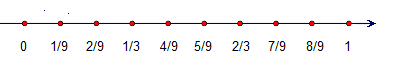
If we draw a number line and mark rational numbers then two things catch the eye:

• no matter how close we look, there will always be infinitely many rational numbers between any two chosen rational ones
• no matter how close we look, there will always be infinitely many irrational numbers between any two chosen rational ones

The rational numbers have gaps, the number line does not. The question is thus: how do we fill the gaps between $\mathbb{Q}$ and $\mathbb{R}$? One method to achieve this goal was presented by Julius Wilhelm Richard Dedekind (1831 – 1916) via so-called Dedekind cuts that are based on the observation, that we can precisely locate any gap between rational numbers by telling which rational numbers are to the left of it and which are to the right of it. This method basically follows the intuition of the geometrical view of the number line. Another method that is the preferred one nowadays was presented by contemporary Georg Ferdinand Ludwig Philipp Cantor (1845 – 1918). This method is analytical. It doesn’t look at what is outside a gap, it describes what is in a gap, i.e. where we end up when we consider endlessly nested intervals. E.g.
$$
\sqrt{2}=1.414213562373095048801688724209 \ldots
$$
which means it is between
\begin{align*}
1&\text{ and } 2\\
1.4=\dfrac{14}{10}&\text{ and } 1.5=\dfrac{15}{10}\\
1.41=\dfrac{141}{100}&\text{ and } 1.42=\dfrac{142}{100}\\
1.414=\dfrac{1414}{1000}&\text{ and } 1.415=\dfrac{1415}{1000}\\
1.4142=\dfrac{14142}{10000}&\text{ and } 1.4143=\dfrac{14143}{10000}\\
&\;\ldots
\end{align*}
These intervals become shorter and shorter. And there is only one number, $\sqrt{2},$ that is contained in all intervals. We write
$$
\sqrt{2}\in \left[\dfrac{a_n}{10^n},\dfrac{b_n}{10^n}\right] \text{ for all }n\in \mathbb{N} \Longrightarrow \lim_{n \to \infty}\dfrac{a_n}{10^n}=\lim_{n \to \infty}\dfrac{b_n}{10^n}=\sqrt{2}
$$
which means that $\sqrt{2}$ is the limit of the interval borders. The borders get narrower and narrower, and so do the distances between $a_n/10^n$ and $a_{n+1}/10^{n+1}$ and likewise between $b_n/10^n$ and $b_{n+1}/10^{n+1}.$ Sequences with this property are called Cauchy sequences, named after Augustin-Louis Cauchy (1789 – 1857). So all we have to do to get all real numbers (up to some technical details) is to add all limits of rational Cauchy sequences
$$
\mathbb{R}=\left\{\left.r\, \right| \,\text{ there is a Cauchy sequence }(C_n)_{n\in \mathbb{N}}\subseteq \mathbb{Q}\text{ such that }\lim_{n \to \infty}C_n=r\right\}.
$$
It is called the topological completion of the rational numbers since it fills all the gaps on the number line that are not rational numbers. We construct the real numbers in a way that guarantees the existence of those limits.

Note that we did not define the real numbers by their decimal representation! $\sqrt{2}=1,414213562373095048801688724209 \ldots$ is not a real number since we cannot write it down to the end. It will always be a rational number. The dots indicate that it goes on forever. It is the limit that is hidden in the dots. E.g.
$$
0.999999\ldots =0.\overline{9}=\sum_{k=1}^\infty \dfrac{9}{10^k}=\lim_{n \to \infty} \underbrace{\sum_{k=1}^n \dfrac{9}{10^k}}_{=a_n}=\dfrac{1}{1-(9/10)}-9=1
$$
The decimal representation is only a tool that allows us to communicate. The real number it represents is the limit. The different representation of one by $0.999999\ldots$ on one hand and $1$ on the other is what I meant by technical details. It means that mathematical rigor requires some additional arguments to match the two representations.

Algebraic Closure

We began our journey by solving the equations $a+x=b$ and $a\cdot x=b.$ Then we used geometrical methods to define the number line. Yet, there are still equations we cannot solve:
$$
x^2+1=0.
$$
This polynomial equation has no rational or real solutions. However, we already know what has to be done to add zeros of polynomials
$$
\mathbb{Q}\subseteq \mathbb{R}\subseteq \mathbb{R}( i )
$$
where $i$ solves $x^2+1=0.$ Similar to the procedure we used for $\sqrt{2},$ we now get the complex numbers
$$
\mathbb{C}= \mathbb{R}(i)=\mathbb{R} + i\cdot \mathbb{R}.
$$
It was more or less already known to the Babylonians that
$$
x^2+px+q=0 \text{ implies } x= \dfrac{1}{2}\left(-p\pm \sqrt{p^2-4q}\right)
$$
and that the root cannot be solved in any case. The crucial point by naming $\sqrt{-1}= i$ is that we can calculate with it without even knowing what it is, simply by respecting $i^2 =-1.$
It is a non-real solution, an imaginary number. But what makes $i$ so special in comparison to all other algebraic numbers we already captured on the real number line? Yes, it is not on the line, so we found an example of a missing algebraic number. Are there more of them that we have to take into consideration? The answer to this question is no, and this is what makes $i$ so special.

Every complex polynomial has a complex zero.

This theorem is so important that it is called the fundamental theorem of algebra. But what makes it fundamental? It is the long division that makes it. Say we have a complex polynomial $p_0(x)\in \mathbb{C}[x]$ and a complex zero $p_0(a_0+ib_0)=0.$ Then we can write
$$
p_0(x)=p_1(x)\cdot (x-(a_0+ib_0)) \text{ with } \deg p_1(x) < \deg p_0(x)
$$
We now proceed by the next zero, a zero of $p_1(x),$ and reduce the degree again and proceed until we end up with a linear polynomial and
$$
p_0(x)=(x-(a_0+ib_0))\cdot(x-(a_1+ib_1))\cdot\ldots\cdot (x-(a_n+ib_n))
$$
By simply adding the imaginary unit $i,$ we are able to solve all complex polynomial equations, i.e. there are no algebraic numbers left to add. The complex numbers are algebraically closed.

Quaternions and Octonions

The complex numbers can be visualized as points in the complex plane because $\mathbb{C}=\mathbb{R}+i\cdot\mathbb{R},$ and Sir William Rowan Hamilton (1805 – 1865) spent years figuring out a similar construction for the three-dimensional space. He failed. But at least he found a four-dimensional construction
$$
\mathbb{H}=\mathbb{R}+i\cdot\mathbb{R}+j \cdot\mathbb{R}+k\cdot\mathbb{R}
$$
which we now call Hamilton numbers or quaternions. Unfortunately, he had to give up commutativity. The multiplication table is given by
$$
\begin{array}{|c|c|c|c|c|}
\hline \cdot &\;\,1\;\, &i&j&k\\
\hline \;1\;&1&i&j&k\\
\hline i&i&-1&k&-j\\
\hline j&j&-k&-1&i\\
\hline k&k&j&-i&-1\\
\hline
\end{array}
$$
which is not symmetric. Such a skew field is called a division algebra. Ferdinand Georg Frobenius (1849 – 1917) proved in 1877 that there are only these three associative, finite-dimensional, real division algebras, $\mathbb{R},\mathbb{C},\mathbb{H}.$

Why do we emphasize associativity? It is because there is another finite-dimensional, real division algebra if we drop the requirements of a commutative and an associative multiplication, the Cayley numbers or octonions. They have eight dimensions over the real numbers and are a non-associative extension of the quaternions. Octonions were first described by John Thomas Graves (1806 – 1870) in a letter to Sir William Rowan Hamilton in 1843. They were independently discovered and first published by Arthur Cayley (1821 – 1895) in 1845,
$$
\mathbb{O}=\mathbb{R}+i\cdot \mathbb{R}+j\cdot \mathbb{R}+k\cdot \mathbb{R}+l\cdot \mathbb{R} +m\cdot \mathbb{R}+n\cdot\mathbb{R}+o\cdot \mathbb{R}.
$$

Characteristic

The octonions are basically the end of this line. They represent the borderline between fields of characteristic zero and structures called algebras. The line isn’t quite sharp as the notation of division algebras suggests. Algebras are rings that are also vector spaces and there are many of them, e.g. Boolean, genetic, Clifford, Jordan, Graßmann, Lie, or – for string theory physicists – Virasoro algebras, etc. Wait! What does characteristic mean? We have used $1\neq 0$ so far which makes sense since otherwise, every calculation would result in zero. But what happens if set
$$
\underbrace{1+1+1+\ldots+1+1}_{n\text{ times}}=0,
$$
which is not as far-fetched as it sounds since $1+1=0$ within our field of light switch states $\{0,1\}.$

Another example would be the twelve-hour mark on the face of a clock. If we consider $1$ as $+1$ hour, then $1+1+1+1+1+1+1+1+1+1+1+1=0.$ However, we have
$$
3\cdot 4 = 0\text{ and }2\cdot 6 = 0
$$
in that case which doesn’t allow us a division by $2,3,4$ or $6,$ if we still want $1\neq 0.$ On the other hand, if we have a prime $p$
$$
\underbrace{1+1+1+\ldots+1+1}_{p\text{ times}}=p=0,
$$
then we won’t get into that trouble. Such a set would consist of $p$ many elements and in fact, represents a field in which we can perform all four basic operations,
$$
\mathbb{F}_p=\{0,1,2,\ldots,p-1\}.
$$
We call $p$ the characteristic of $\mathbb{F}_p.$ In case $p=\infty ,$ i.e. sums of ones will never be zero as in our usual fields $\mathbb{Q},\mathbb{R},\mathbb{C},$ we say that the characteristic of such fields is zero. This is a convention because mathematicians do not like to consider infinity as a number. However, they have no problem calling characteristics $p$ finite in order to distinguish them from $0.$ All fields $\mathbb{F}_p$ are prime fields because they only consist of the minimum of necessary elements, and the light switch is
$$
\mathbb{F}_2=\{[\text{ ON }],[\text{ OFF }]\}=\{0,1\}.
$$
A field of characteristic $p=2$ has no signs
$$
1+1=0 \text{ implies } 1=-1.
$$
This is especially important in all cases where signs play a crucial role; e.g. for Graßmann or Lie algebras!

Algebraic and transcendental extensions can be constructed just as in the case of the rational numbers. But the identification $p=0$ has a funny consequence
$$
(x+y)^p=\sum_{j=0}^p \binom{p}{j} x^{p-j}y^j=x^p+p\cdot x^{p-1}y+\ldots+p\cdot xy^{p-1}+y^p=x^p+y^p.
$$

p-adic Numbers

The absolute value of a number on the number line measures its distance from zero. It is called a valuation, an Archimedean valuation to be exact. This means that we can always put the smaller length together so many times that it exceeds the larger length.
$$
|N \cdot a|>|b|>|a|>0\quad (N\in \mathbb{N})
$$
Kurt Hensel (1861 – 1941) presented in 1897 a field extension of the rational numbers for which this isn’t true any longer. We are, despite the title of this section, back in the characteristic $0$ case again as the rational numbers will be our prime field. Say we have a prime $p$ and $a=p^r \cdot m’\; , \;b = p^s \cdot n’.$ Then
$$
\left|\dfrac{a}{b}\right|_p = \begin{cases}  p^{-r+s} &\text{ if } a \neq 0\\ 0&\text{ if }a=0\end{cases}
$$
defines a valuation that is no longer Archimedean. Nevertheless, it still defines a distance by
$$
d(a,b)=|a-b|_p.
$$
With the distance comes the opportunity of a topological completion, the $p$-adic numbers
$$
\mathbb{Q}_p=\left\{\left.\dfrac{a}{b} \right| \text{ there is a Cauchy sequence }(C_n)_{n\in \mathbb{N}}\subseteq \mathbb{Q}\text{ such that }\lim_{n \to \infty}C_n=\dfrac{a}{b}\right\}
$$
It is the same definition as for the real numbers, but with a different distance and thus establishing a different calculus. This means we are dealing with an ordering that can no longer be visualized by a number line, e.g.
$$
\left|\dfrac{1}{2^n}\right|_5=\left|3^n\right|_5=1\; \;,\; \;
\left|5^n\right|_5=\dfrac{1}{5^n}\;\; ,\;\;\left|10\right|_5= \left|15\right|_5=\left|20\right|_5=\dfrac{1}{5}
$$
Helmut Hasse (1898 – 1979) showed in his dissertation 1921 about quadratic forms that rational equations can be solved – up to many complicated technical details – if they can be solved for real numbers and all p-adic numbers. This makes $p$-adic numbers interesting for algebraic number theory. His dissertation established an entire branch of mathematics. For example, O’Meara’s textbook ‘Introduction to Quadratic Forms‘ has $342$ pages!

Continuum Hypothesis

We have finite prime fields $\mathbb{F}_p$ and the countable infinite rational numbers $\mathbb{Q}.$ Countable means that the rational numbers can be enumerated
$$
\begin{array}{cccccccccccc}
0 &\to &\frac{1}{1} &\to &\frac{1}{2}&&\frac{1}{3}&\to&\frac{1}{4}&&\frac{1}{5}&\to \\
&&&\swarrow &&\nearrow &&\swarrow &&\nearrow && \\
& &\frac{2}{1} & &\frac{2}{2}&&\frac{2}{3}& &\frac{2}{4}&&\frac{2}{5}& \ldots \\
&&\downarrow&\nearrow&&\swarrow&&\nearrow&&&&\\
& &\frac{3}{1} & &\frac{3}{2}&&\frac{3}{3}& &\frac{3}{4}&&\frac{3}{5}& \ldots \\
&&&\swarrow&& \nearrow&&&&&\\
& &\frac{4}{1} & &\frac{4}{2}&&\frac{4}{3}& &\frac{4}{4}&&\frac{4}{5}& \ldots \\
&&\downarrow&\nearrow&&&&&&&\\
& &\frac{5}{1} & &\frac{5}{2}&&\frac{5}{3}& &\frac{5}{4}&&\frac{5}{5}& \ldots \\
& &\vdots & &\vdots&&\vdots& &\vdots&&\vdots& \ldots
\end{array}
$$
Uncancelled quotients can be omitted in order to avoid double enumeration. In order to enumerate the negative rational numbers, too, we could e.g. count positive rational numbers by even numbers and negative rational numbers by odd numbers. The scheme above shows only positive ones for simplicity.

Finite fields remain finite, and the rational numbers remain countable infinite if we construct field extensions with finite many algebraic numbers. We get countable infinite fields from both if we construct field extensions with finite many transcendental numbers. Remember that a transcendental field extension is the same as adding an indeterminate variable $x$ and its integer powers.

It is the topological completion that makes the step countable to uncountable. The real numbers are an uncountable infinite set. This can easily be seen. Imagine that we have an enumeration of the real numbers, say between $\pm 9$

$$
\begin{array}{ccc}
a_1&=&+\underline{0}.1234567890123456\ldots\\
a_2&=&+2.\underline{7}182818284590452\ldots\\
a_3&=&+3.1\underline{4}15926535897932\ldots\\
a_4&=&+0.00\underline{0}0000000000000\ldots\\
a_5&=&-1.000\underline{0}000000000000\ldots\\
a_6&=&+1.4142\underline{1}35623730950\ldots\\
a_7&=&+2,66514\underline{4}1426902251\ldots\\
a_8&=&+0,083333\underline{3}333333333\ldots\\
a_9&=&+0,5772156\underline{6}49015328\ldots\\
a_{10}&=&-1,61803398\underline{8}7498948\ldots\\
\vdots&:&\vdots
\end{array}
$$
We underlined the diagonal elements because we construct a number $d_1.d_2d_3d_4\ldots$ from the digits on the diagonal by setting
$$
d_k:=\begin{cases}0 &\text{ if }a_{kk}\neq 0\\ 2&\text{ if } a_{kk}=0\end{cases}
$$
This produces a number $2.002200000\ldots$ that cannot be enumerated by our scheme since it differs from all enumerated numbers in at least one digit. Hence, $\mathbb{R}$ is uncountable and infinitely large. The size of a set is called its cardinality. Equal cardinalities of two different sets mean that there is a bijection between the sets, a mapping between the elements of the sets that is unique in both directions. The enumeration of the rational numbers is such a mapping between $\mathbb{N}$ and $\mathbb{Q}.$ The cardinality of $\mathbb{N},$ countable infinity, is abbreviated by the Hebrew letter for a,
$$
|\mathbb{N}|=\aleph_0.
$$
The cardinality of the set of all subsets of $\mathbb{N}$ is, therefore, $2^{\aleph_0}$ which is also the cardinality of the real numbers and the real interval $[0,1],$ short: the cardinality of the continuum
$$
|\mathbb{R}|=|[0,1]|=|\{S\,|\,S\subseteq \mathbb{N}\}|=2^{\aleph_0}
$$
The lowest cardinality bigger than $\aleph_0$ is noted as $\aleph_1.$ One could suppose that it will be that of the continuum. This is called the continuum hypothesis:

There is no uncountable infinite set of real numbers whose cardinality is smaller than that of the set of all real numbers.

that is

There is no set whose size lies between the size of the natural numbers and the size of the real numbers.

or in the formulation, Kurt Friedrich Gödel (1906 – 1978) used it

Every infinite subset $M$ of the real numbers is either of equal size as $\mathbb{R}$ or $\mathbb{N}$.

True is that we cannot know! Our current set theory remains valid with the assumption that the continuum hypothesis is true, as well as with the assumption that the continuum hypothesis is false.
$$
2^{\aleph_0}\stackrel{?}{=}\aleph_1
$$