Fun with Self-Avoiding Walks Simulations

This post is about some simulations I did of self-avoiding random walks. These are what they sound like with each step, the position of the walk moves randomly, with the constraint that it can’t visit the same spot more than once. These are mathematically somewhat interesting and crop up in a few areas of physics; I was simulating them because I thought they would solve an unknown problem in polymer physics that I had encountered in my PhD.

Key Points

1. Self–avoiding random walks are simulations that move randomly but don‘t visit the same spot more than once
2.  The Flory free energy combines entropic elasticity and excluded volume to calculate the excess energy cost of not having particles overlap
3. The ideal chain grows as ##R \approx L^{0.5}## and the swollen chain grows as ##R\approx L^{0.6}##
4. Semi–flexibility can interfere with excluded volume by making it less likely for two nearby segments of a molecule to bump into each other, and this changes the statistics of the chain
5. The blob model says that a chain can be imagined as a 2D self–avoiding walk of spherical blobs, inside each of which the chain does a 3D self–avoiding walk
6. As you cram DNA in narrower and narrower slits, the molecule spreads out more and more according to the negative quarter–power of the height of the slit
7. My simulation of self–avoiding random walks approaches the asymptotic behaviour of the self–avoiding walk
8. Plugging in some of the numbers from my simulations, I can predict a scaling of –0.2 instead of –0.25, closer to the experimental result of 0.16

The Simulation

The simulations work as follows: on a square lattice, starting at the origin, take a step in a random direction. If that direction is occupied, try another direction. If all directions are filled, stop. Aficionados of the video game Snake may recognize this halting condition. The shortest distance it can travel before trapping itself is eight steps (this happens in the gif if you watch carefully), and the average number of steps it travels before stopping is about 70. The main parameters I was measuring were the distance between the two ends, and the radius of gyration, which is essentially the standard deviation of the position of each site (the centre of mass is the mean of each site, the radius of gyration is the root-mean-square displacement of each site from the centre of mass). I was interested in how the radius of gyration grows with the number of steps.

The Wikipedia page gives some examples of their applications in physics and math. An interesting one is that it’s equivalent to the Ising model (interacting magnetic spins on a lattice) with zero degrees of freedom. I have also read a paper comparing the enumeration of self-avoiding walks to the entropy of a black hole surface, which I’d like to learn more about. There’s also an entire book on the subject. I want to mainly discuss them in the context of polymer physics.

A polymer is a long stringy molecule, and the simplest way to model it is as a random walk through space. My second blog post introduces a few of the physical phenomena that polymer chains exhibit, which typically involve maximizing entropy by contracting into blobs. The “ideal chain” model of a polymer has no interactions between different segments of the chain, and no long- or short-range correlation in orientation along the chain, which is why it is described by the random walk. The average distance travelled by a random walk is zero, and the average distance between the two ends of a polymer is zero. However, the mean-square displacement (MSD) of a random walk is non-zero, and the mean-square end-to-end distance is non-zero. The MSD is proportional to the number of steps in the walk, so the root-mean-square (RMS) displacement is proportional to the square root of the number of steps. For an ideal polymer, the end-to-end distance and radius of gyration is proportional to the square root of the length of the chain. In the language of scaling laws, $R_{g}\approx L^{0.5}$.

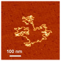This polymer on a surface totally looks like a random walk! From JACS 124, 13454.

However, in reality, no two segments of a polymer chain can occupy the same point in space. This means, that instead of being described by the random walk, it is described by the self-avoiding random walk. Because the self-avoiding walk excludes configurations that visit the same site, it is generally bigger than a self-avoiding walk of the same length: if you “turn on” self-avoidance interactions, the chain “swells” so this is called a swollen chain. So, if the ideal chain grows as $L^{0.5}$, how does the swollen chain grow with length?

If we consider some number N particles each with volume v inside a larger volume V, the probability of any two particles occupying the same space is

$$p_{1}=\frac{v}{V}$$

So the probability of them not occupying the same space is:

$$\overline{\,p_{1}}=1-\frac{v}{V}$$

Now, if there are N of these particles, there are N(N-1)/2 pairwise combinations of them, so the probability of no two particles occupying the same space is:

$$\overline{\,p_{N}}=\left(1-\frac{v}{V}\right)^\frac{N(N-1)}{2}$$

Rewriting this and then assuming that N is big, we have

$$\overline{\,p_{N}}=exp\left[\frac{N(N-1)}{2}\log{\left(1-\frac{v}{V}\right)}\right] \approx exp \left[-N^{2}\frac{v}{V}\right]$$

The approximation arises from the Taylor expansion of log(1-x) as well as the fact that N-1 is roughly N. I also dropped a factor of two, because it makes me feel powerful to do that. Now, we take a lesson from the canonical ensemble and remember that according to the Boltzmann distribution, the probability of observing the system in some state is exponentially decaying with the energy of that state. Our probability is already exponentially decaying, so it tells us the excess energy cost of not having the particles overlap due to excluded volume (EV):

$$E_{EV}\approx kT\cdot N^{2}\frac{v}{V}\approx kT\cdot N^{2}\frac{v}{R^3}$$

Here, kT is the thermal energy, and I assumed that we live in three dimensions, which isn’t a necessary one. This is half the picture. The other half is entropy: a random walk is more likely to be observed in a high-degeneracy state. A random chain is unlikely to be in an extended state; the ends are statistically more likely to be found close to each other. The size of a random walk, being random, has a Gaussian distribution, and through the Boltzmann distribution, this gives rise to entropic elasticity: the energy of extending an ideal chain is harmonic, and the spring constant is its average radius of gyration, which is the product of the step size and the number of steps N.

When we combine these two factors, entropic elasticity and excluded volume, what we’re essentially calculating is the excess energy due to the loss of entropy when you exclude states that don’t overlap. This is known as the Flory free energy.

$$E_{F}=kT\left(\alpha \frac{R^2}{N}+ \beta \frac{N^3}{R^3}\right)$$

I’m interested in how R and N scale with one another, so I’ve dropped all other coefficients and embedded them in Greek prefactors. If we take the derivative of the Flory energy and minimize it concerning the chain radius of gyration, we find:

$$\frac{dE}{dR}=kT\left(2\alpha \frac{R}{N}-3\beta \frac{N^3}{R^4}\right)=0 \rightarrow R \approx N^{\frac{3}{5}}$$

So, we have derived the scaling relation of the swollen chain. The ideal chain grows as $R \approx L^{0.5}$ and the swollen chain grows as $R\approx L^{0.6}$. After 10 steps, the swollen chain will be 25% bigger, after 1000 steps it will be twice as big. Through some trickery involving the renormalization group that I don’t understand, the exponent is closer to 0.588 rather than 0.6. You can also replace the three-dimensional volume $R^3$ with some arbitrary dimension $R^d$ to get a more general result. For the two dimensions, in which I did my simulations, it is 3/4 instead of 3/5.

Neat derivation, but why did I do those simulations I showed at the beginning? My PhD research was part of a field that uses DNA molecules to test the predictions of polymer physics. An early experiment in this field looked at the diffusion coefficient of different-sized DNA molecules and found that the growth exponent was experimentally consistent with 0.588, the wormlike chain. However, there’s an additional effect I haven’t talked about called semi-flexibility, which has to do with the fact that polymers are rigid over short distances. For synthetic polymers, this is typically a length so short as to be negligible, but for DNA it’s about 50 nanometers, much larger than the double-helix diameter of about 2 nanometers. Semi-flexibility can interfere with excluded volume by making it less likely for two nearby segments of a molecule to bump into each other, and this changes the statistics of the chain. A general gap of knowledge in polymer physics is what happens when you combine semi-flexibility with excluded volume.

Is DNA a good model polymer?

In 2013, the ungoogleable Douglas Tree and some co-authors (including my current supervisor) wrote a paper called “Is DNA a good model polymer?” and according to Hinchcliffe’s Rule you can guess what the answer is. They did simulations of semi-flexible chains with excluded volume; essentially a much more nuanced version of the gif I’ve shown on top, in three dimensions. They measured how the end-to-end distance depends on length for a swollen semiflexible chain and looked at the logarithmic derivative of this trend, which is essentially the “local” Flory exponent at that particular length. For short chains, because they are effectively rigid, they grow linearly in separation with length, and the Flory exponent is close to 1.0 for the shortest chains. For very long chains, they act like self-avoiding walks with a Flory exponent asymptotically approaching 0.588. However, for intermediate length chains, things get tricky, because it’s some combination of short-chain rod behaviour, long-chain excluded volume behaviour, and the fact that medium-length chains are less likely to bump into each other than long ones. The DNA that people tend to use for experiments, which comes from viral genomes, is right in this intermediate range of lengths where no limiting theory works.

This was the most interesting paper I read that year, and it made me think because my research was trying to verify all these theories that assume infinitely long chains. Some aspects of my data didn’t agree with the theory, so was my data wrong, or was the theory wrong because the molecules it was attempting to describe were too short?

One aspect of this involved DNA confined in a slit smaller than its radius of gyration, narrow enough to make the molecule behave as if it were in two dimensions. There have been several experiments looking at DNA confined in slits and seeing how the “spread” of the molecule depends on the height of the slit.

 

DNA spreads out more in narrower slits. Images from here, cartoons by me.

The theory that predicts the spread of a chain in slit confinement works by renormalizing the chain into spheres that fill up the slit, called blobs. Inside each blob, the chain undergoes a self-avoiding walk in three dimensions, with a Flory exponent of 0.6. The renormalized chain of blobs undergoes a self-avoiding walk through the slit in two dimensions, with a Flory exponent of 0.75. You can figure out how big the two-dimensional random walk is by figuring out how much of the chain gets repackaged into each blob, and how many blobs there are. So, if the blob is the same size as the height of slit, h, the number of blobs is the total chain length divided by the length of chain in each blob, and the length of chain in each blob obeys 3D Flory statistics, you can figure out that:

$$R(h)\approx h^{1-\frac{0.75}{0.6}}\approx h^{-0.25}$$

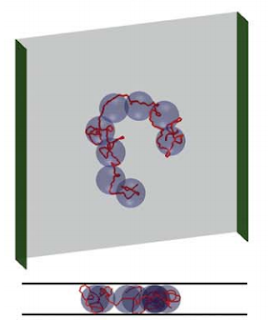The blob model says that a chain can be imagined as a 2D self-avoiding walk of spherical blobs, inside each of which the chain does a 3D self-avoiding walk. Image from here.

This is saying that as you cram DNA in narrower and narrower slits, the molecule spreads out more and more according to the negative quarter-power of the height of the slit. The problem was that experiments testing this did not find a result that agreed with this prediction (or with each other, but that’s a different issue).

My idea to resolve this discrepancy was that the chains weren’t long enough to behave like a 2D self-avoiding walk, as Tree and Friends showed in 3D. There is a good reason to suspect this because if you look at pictures of DNA in narrow slits, you will see that it doesn’t encounter itself that often. So, inspired by the 3D simulations of semi-flexible self-avoiding walks, I wrote my simulation of 2D self-avoiding walks.

Let’s have another look.

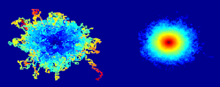
If you look at the aggregate of 10,000 iterations of this algorithm, each of which runs until the molecule traps itself, it looks like the Flying Spaghetti Monster. If you look at a probability density plot of how likely each site is to be visited, it looks like a volcano or the Eye of Sauron.

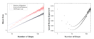
For each step of the self-avoiding walk, I calculated the radius of gyration and the end-to-end distance and kept track of the data as a function of the number of steps. Looking at how these parameters grow with length, we generally recover the 3/4 scaling predicted by Flory theory (a power-law fit gets 0.72).

Left: Simulation results of the size of a self-avoiding walk versus the number of steps it takes. Right: The logarithmic derivative of that size relative to the number of steps, the local scaling exponent.

However, if we look at the logarithmic derivative, d log R/d log N, we can see how it approaches this asymptotic limit with length. It is similar to the 3D case. Starting from the rod-like limit (when you go from one to two steps, it can only double in size) it falls towards the ideal 0.5, reaching a minimum and then rising towards 0.75. My data isn’t quite enough to reach that limit, and there’s this weird even-odd pattern which I believe is caused by the fact that I discretize the walks to a square lattice. Because walks longer than length 70 get relatively rare, the noise in the simulation picks up after that point.

This possibly suggests a correction to the standard Flory prediction for a molecule’s size in a slit, but the problem is that the same derivation doesn’t work because it assumes that these scaling relations hold, and you can’t change some of the numbers without really changing the whole form of the equation. Plugging in some of the numbers from my simulations, I can take the minimum exponent which is about 0.65 and the minimum 3D exponent from Tree’s paper, which is about 0.54, I predict a scaling of about -0.2 instead of -0.25. This is closer to the experimental result of about 0.16 but still doesn’t fit the data, and isn’t physically justified.

Conclusion

I stopped working on this particular research avenue shortly after figuring this out, but it was kind of fun creating this random walk simulation and seeing how it approaches the asymptotic behaviour of the self-avoiding walk. This was a fairly long and rambly story about why I was doing these simulations. Just to summarize, I started simulating self-avoiding random walks because I thought that an unknown aspect of their behaviour, the asymptotic growth of their Flory exponent, would resolve some standing questions in polymer physics. It didn’t, but I tried.

Click For Forum Comments