Learn About the Greenberger-Horne-Zeilinger Experiment

In two previous Insights, I shared Mermin’s explanation of the Hardy experiment[1] and the Mermin device[2]. Both of his corresponding AJP papers presented nontechnical arguments against “instruction sets” aka “counterfactual definiteness” for quantum mechanics (QM). In the case of the Mermin device, Elitzur & Dolev showed a particular experimental instantiation yielded a quantum counterpart to the liar paradox[3]. Herein I will share a third Mermin AJP paper[4] against counterfactual definiteness in QM, i.e., a nontechnical version of the Greenberger-Horne-Zeilinger (GHZ) experiment[5]. I will then provide the corresponding QM formalism, which Dowker uses to motivate Sorkin’s Many Histories interpretation of QM[6].

Mermin’s GHZ device is shown in his Figure 1 below. The three experimentalists may choose either setting 1 or setting 2 at detectors A, B, and C, and will find one of two outcomes, i.e., red (R) or green (G), in each trial/run of the experiment. As with the Mermin device, I will provide QM formalism using spin (it has been done using photons[7]), but Mermin’s explanation of “no instruction sets” can be understood without the QM formalism. Here are the interesting results of the experiment, i.e., those that are incompatible with the existence of instruction sets:

1. If one detector is set to 1 and the others are set to 2, then an odd number of red lights always flash (RRR, RGG, GRG, and GGR occur with equal frequency).
2. If all three detectors are set to 1, then an odd number of red lights never flash (two of three flash R or all flash G).

Let me once again present the standard arguments for “local realism” (that Mermin attributes to Einstein, Podolsky, & Rosen[8]). The particles don’t ‘know’ how they will be measured in any given run, in fact the detector settings can be chosen an instant before the particles arrive at their respective detectors. And, assuming the measurements are space-like separated, no information about the setting and outcome at one detector can reach the other detectors before the particles are measured there, i.e., the measurements are said to be “local.” Thus, the particles don’t ‘know’ how they will be measured when they are emitted and they can’t transmit that information to each other during the run. So, it seems the particles’ possible outcomes with respect to each possible detector setting must be coordinated to guarantee the outcomes shown in results 1 and 2 above.  Mermin calls the coordination of outcomes “instruction sets” and the fact that the particles have definite properties corresponding to possible measurements whether they are carried out or not is called “realism” or “counterfactual definiteness.” The combination of these assumptions is often called “local realism” or “Einsteinian local realism”[9]. Both assumptions seem reasonable, locality because the temporal order of space-like separated events is frame dependent according to special relativity, which would seem to rule out superluminal information transfer, and realism because the particles don’t ‘know’ how they will be measured until the last moment and they have to guarantee the outcomes in results 1 and 2 above. So, let’s look at the runs where the settings are 122, 212, or 221 for result 1.

If we’re watching one of the detectors far from the other two, so that we have those results before our detector registers, we will know the outcome at our detector before it registers. This is because we must have an odd number of R outcomes for these settings, so if the other two are RR or GG, our detector must be R. If the other two are RG or GR, then our detector must be G. Since this logic applies to any of three detectors, Mermin concludes there must be an instruction set for each particle for each of the two possible settings. Now let’s see if we can construct an instruction set that makes the above results hold.

For example, the set $\begin{smallmatrix}R & G & G\\G & R & R \end{smallmatrix}$ gives RRR for setting 122, GGR for setting 212, and GRG for setting 221. So, it’s a valid instruction set for result 1. In order to create all the valid sets for result 1, i.e., for the settings 122, 212, and 221, we start with those for 122:

\begin{equation} \begin{smallmatrix} R & – & -\\- & R & R \end{smallmatrix} \mspace{35mu} \begin{smallmatrix} R & – & -\\- & G & G \end{smallmatrix}\mspace{35mu} \begin{smallmatrix} G & – & -\\- & R & G \end{smallmatrix}\mspace{35mu} \begin{smallmatrix} G & – & -\\- & G & R \end{smallmatrix} \label{sets1} \end{equation}

Now if you look at the four sets of Eq(\ref{sets1}) and ask how we can fill in blanks to make the setting 221 produce an odd number of R flashes, we see that there are two ways for each set. For example, $\begin{smallmatrix} R & – & -\\- & R & R \end{smallmatrix}$ can become $\begin{smallmatrix} R & – & R\\R & R & R \end{smallmatrix}$ or $\begin{smallmatrix} R & – & G\\G & R & R \end{smallmatrix}$, so that the setting 221 gives RRR or GRG, respectively. Finally, we have to ask how we can fill in the last blank so that the setting 212 gives an odd number of R flashes and we see that there is only one way to do that in each of our eight cases. For example, $\begin{smallmatrix} R & – & R\\R & R & R \end{smallmatrix}$ must become $\begin{smallmatrix} R & R & R\\R & R & R \end{smallmatrix}$ and $\begin{smallmatrix} R & – & G\\G & R & R \end{smallmatrix}$ must become  $\begin{smallmatrix} R & G & G\\G & R & R \end{smallmatrix}$  so that the setting 212 gives RRR or GGR, respectively. Thus, there are only eight possible instruction sets to guarantee result 1 above:

\begin{equation} \begin{smallmatrix} R & R & R\\R & R & R \end{smallmatrix} \mspace{35mu} \begin{smallmatrix} R & G & G\\R & G & G \end{smallmatrix}\mspace{35mu} \begin{smallmatrix} G & R & G\\G & R & G \end{smallmatrix}\mspace{35mu} \begin{smallmatrix} G & G & R\\G & G & R \end{smallmatrix}\mspace{35mu} \begin{smallmatrix} R & G & G\\G & R & R \end{smallmatrix} \mspace{35mu} \begin{smallmatrix} R & R & R\\G & G & G \end{smallmatrix}\mspace{35mu} \begin{smallmatrix} G & G & R\\R & R & G \end{smallmatrix}\mspace{35mu} \begin{smallmatrix} G & R & G\\R & G & R \end{smallmatrix}  \label{sets2} \end{equation}

And now you can see we’re in trouble because we also need result 2 to hold and that says the setting 111 never produces an odd number of R flashes. But, in every one of the eight instruction sets of Eq(\ref{sets2}), the only collection that will produce an odd number of R flashes for 122, 221, or 212 settings per result 1, we will get an odd number of R flashes for the setting 111. And, what’s to prevent two of the experimentalists from changing their setting 2 to setting 1 at the last split second? So, as with the Mermin device and the Hardy experiment, instruction sets (aka counterfactual definiteness) just don’t work. Now let’s look at the consequence of this as we did with the quantum liar experiment for the Mermin device.

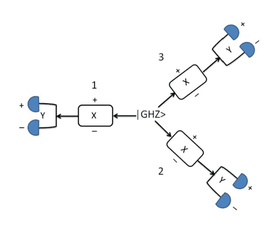
In Dowker’s GHZ set-up (Figure 2), the GHZ spin state $\mid \Psi \rangle = \mid +++ \rangle + \mid -\: -\: – \rangle$ (in the eigenbasis of $\sigma _z$) proceeds from the Source through three Stern-Gerlach (SG) magnets oriented in the x direction, but with no detectors following (although, we may choose to do an x measurement there if we wish). If no x measurement is made, each possible outcome at each SG x magnet (where no measurement was made) is recombined then redirected to a SG magnet oriented in the y direction where a measurement is made. She then reasons as follows.

The GHZ state is an eigenstate of the following four operators:

\begin{equation} \begin{split} P &= \sigma _x \sigma _y \sigma _y \\ Q &= \sigma _y \sigma _x \sigma _y \\ S &= \sigma _y \sigma _y \sigma _x \\ X &= \sigma _x \sigma _x \sigma _x \label{operators} \end{split} \end{equation}

Letting setting 1 correspond to x and setting 2 correspond to y, we will see that these four operators are just giving various multiplicative results of the three outcomes in the trials for results 1 and 2 above. To find the eigenvalues of P, Q, S, and X,  we need to find the action of $\sigma _x$ and  $\sigma _y$ on the eigenvectors of $\sigma _z$. In a previous Insight I used

\begin{equation} \sigma _z = \begin{pmatrix} 1 & 0\\0 & -1 \end{pmatrix}   \label{spinz} \end{equation}

and

\begin{equation} \sigma _x = \begin{pmatrix} 0 & 1\\1 & 0 \end{pmatrix}   \label{spinx} \end{equation}

in the eigenbasis of $\sigma _z$. Since the eigenvectors of $\sigma _z$ are simply $\mid + \rangle = \begin{pmatrix} 1\\0 \end{pmatrix}$ for spin up (eigenvalue = +1) and $\mid – \rangle = \begin{pmatrix} 0\\1 \end{pmatrix}$ for spin down (eigenvalue = -1), we see $\sigma _x \mid + \rangle =\: \mid – \rangle$ and $\sigma _x \mid – \rangle =\: \mid + \rangle$ from explicit matrix multiplication. To find the action on these vectors by $\sigma _y$ we need $\sigma _y$ in the eigenbasis of $\sigma _z$

\begin{equation} \sigma _y = \begin{pmatrix} 0 & -i\\i & 0 \end{pmatrix}   \label{spiny} \end{equation}

So, $\sigma _y \mid + \rangle = i\mid – \rangle$ and $\sigma _y \mid – \rangle = -i\mid + \rangle$, which we can see from explicit matrix multiplication. Thus,

\begin{equation}  \sigma _x \sigma _y \sigma _y \left( \mid +++ \rangle + \mid -\: -\: – \rangle \right) = (+1)(i)(i)\mid -\: -\: – \rangle + (+1)(-i)(-i)\mid +++ \rangle = -\mid \Psi \rangle \label{Peigen} \end{equation}

which tells us $P\mid \Psi \rangle = -\mid \Psi \rangle$. We likewise find $Q\mid \Psi \rangle = -\mid \Psi \rangle$, $S\mid \Psi \rangle = -\mid \Psi \rangle$, and $X\mid \Psi \rangle = \mid \Psi \rangle$. What does this mean as far as experimental outcomes?

Spin x, y, and z measurements are represented by $\sigma _x$, $\sigma _y$ and $\sigma _z$ with the outcomes given by their eigenvalues. In all three cases, the eigenvalues are +1 and -1. I gave the eigenstates for $\sigma _x$ in the eigenbasis for $\sigma _z$ in a previous Insight, thereby showing its eigenvalues +1 and -1. Those for $\sigma _z$ are trivial and shown above. Those for $\sigma _y$ are $\begin{pmatrix} 1\\i \end{pmatrix}$ with eigenvalue +1 and $\begin{pmatrix} 1\\-i \end{pmatrix}$ with eigenvalue -1. For example,

\begin{equation} \begin{pmatrix} 0 & -i\\i & 0 \end{pmatrix} \begin{pmatrix} 1\\i \end{pmatrix} = \begin{pmatrix} 1\\i \end{pmatrix}    \label{spinyeigen} \end{equation}

This means we obtain $\pm 1$ whenever we measure spin x, y, or z (we’re only measuring x or y in Dowker’s GHZ device). Likewise, when we measure P, Q, S, or X, the result will be their eigenvalues of $\pm 1$ shown above. Combining these two facts we see that Mermin’s GHZ device says settings 122 (P), 212 (Q), and 221 (S) must produce an odd number of R flashes, where R corresponds to a -1 outcome and G corresponds to +1 outcome, so that the multiplicative total of all three x and y spin measurement outcomes is -1, i.e., the eigenvalue of P, Q, and S. Likewise, the 111 setting (X) must produce an even number of R flashes, so that the multiplicative total is +1, i.e., the eigenvalue of X. Thus, we see that the QM formalism reproduces results 1 and 2 above for the Mermin GHZ device which means the Mermin analysis holds, i.e., there are no instruction sets. What is the implication of no counterfactual definiteness in Dowker’s GHZ device?

Individual x and y measurement outcomes $s_x = \pm 1$ and $s_y = \pm 1$ (actual or counterfactual) for each of the three particles at any of the detectors in Figure 2 correspond to a particular path through the apparatus. Let’s write such a collection of outcomes for all three particles as $\Omega =\left( s_x, s_y, s_x, s_y, s_x, s_y \right)$. Since $\Omega$ is a particular set of paths through the device for all three particles from emission at the Source to eventual detection, Dowker and Sorkin refer to it as a “history.” The values in $\Omega$ must satisfy $P = s_xs_ys_y = -1$, $Q = s_ys_xs_y = -1$, $S = s_ys_ys_x = -1$, $X = s_xs_xs_x = 1$, and $PQSX = \left(s_xs_ys_y\right)\left(s_ys_xs_y\right)\left(s_ys_ys_x\right)\left(s_xs_xs_x\right) =\: –1$. Thus, Mermin’s explanation showing the impossibility of an instruction set has the mathematical counterpart here in the impossibility of the last requirement PQSX = -1, since each particle’s $s_x$ and $s_y$ is squared in PQSX. Since each $\Omega$ corresponds to a particular spacetime history (set of three paths) for Figure 2, Dowker concludes that “The physical world cannot be a single history.” This prompts her to ask, “If not a single history, then what?” She then says, “We don’t know the answer to this question, it’s a work in progress.” Since Sorkin’s path integral formalism (quantum measure theory) uses paths, she and Sorkin introduce more than one set of paths to answer the question, i.e., Multiple Histories.

No matter how you might try to account ontologically for no counterfactual definiteness as we’ve seen it presented in the quantum liar experiment, the GHZ experiment, or Hardy’s experiment, for example, it  seems certain that quantum nonlocality[10] in general will entail a serious revision of our Newtonian mechanistic worldview. So, I close my QM Insights with this quote by Bertlmann[11]:

I have a confession: I am not the realist one might expect after reading Bell’s article “Bertlmann’s socks and the nature of reality”; the world in its very foundations is much more abstract than we think with our “anschauliche” (intuitive) concepts, to borrow Werner Heisenberg’s term. My personal feeling is that Bell’s theorem, which reveals an apparent nonlocality in nature, points to a more radical conception whose onset we do not yet have.

 

 

Figure 1: Mermin’s GHZ Device

 

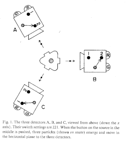
Figure 2: Dowker’s GHZ Set-up

 

Resources

1. Mermin, N.D.: Quantum mysteries refined. American Journal of Physics 62 (10), 880-887 (1994).
2. Mermin, N.D.: Bringing home the atomic world: Quantum mysteries for anybody. American Journal of Physics 49, 940-943 (1981).
3. Elitzur, A., & Dolev, S.: Quantum Phenomena within a New Theory of Time: In: Elitzur, A., Dolev, S., & Kolenda, N. (eds.) Quo Vadis Quantum Mechanics? p 325, Springer, New York (2005).
4. Mermin, N.D.: Quantum mysteries revisited. American Journal of Physics 58, 731-734 (Aug 1990).
5. Greenberger, D.M., Horne, M., & Zeilinger, A.: Going beyond Bell’s theorem: In: Kafatos, M. (ed.) Bell’s Theorem, Quantum Theory, and Conceptions of the Universe, pp 69-72, Kluwer Academic Press, Dordrecht (1989).
6. Dowker, F.: Are there premonitions in quantum measure theory? Presented at “Free Will and Retrocausality in a Quantum World,” Trinity College, Cambridge, 4 July 2014 https://www.youtube.com/watch?v=jETvuojQ2qs
7. Pan, J., Bouwmeester, D., Daniell, M., Weinfurter, H., & Zeilinger, Z.: Experimental test of quantum nonlocality in three-photon Greenberger-Horne-Zeilinger entanglement. Nature 403, 515-519 (3 Feb 2000).
8. Einstein, A., Podolsky, B., & Rosen, N.: Can quantum mechanical description of physical reality be considered complete? Physics 1, 195-200 (1964).
9. Einstein, A.: Considerations Concerning the Fundamentals of Theoretical Physics. Science 91, 487-492 (24 May 1940).
10.  “the phenomenon by which measurements made at a microscopic level contradict a collection of notions known as local realism that are regarded as intuitively true in classical mechanics.” https://en.wikipedia.org/wiki/Quantum_nonlocality
11. Bertlmann, R.: Readers offer their own magic moments with John Bell. Physics Today 68(12), 8-12 (2015).