Learn the Basics of Dimensional Analysis

As a university teacher and as a PF member, I have often noted that students are largely unaware of or not using dimensional analysis to help them in their pursuit of knowledge or to check their results. A number of recent threads on PF have also highlighted this issue. The intent of this Insight is therefore to provide a basic introduction to the subject with a number of examples with which the reader may be familiar. The discussion on the Buckingham pi theorem is a bit more involved and can be skipped without missing the basic concepts.

What is physical dimension?

A common misconception when dimensional analysis is invoked is that students mix up the subject with the number of spatial dimensions, which is not what we want to discuss here. Instead, physical dimensions refer to the type of quantity we are dealing with. It is related to, but not exactly the same as, what units we can use to describe a physical quantity. For example, a length can be measured in centimeters or inches, but an area cannot. Likewise, an area cannot be measured in centimeters or inches but must be measured of squared length units. It would be inconsistent to say that a table had an area of 42 cm, but it could have an area of 1.3 m$^2$. While a centimeter is not the same thing as an inch, they are both examples of units of length. In physics, the physical dimension of a quantity refers to the type of units that must be used to describe it. The basic construction blocks of dimensional analysis are the so-called base dimensions, this is a set of physical dimensions, which to an extent is a matter of convention, that can be used to build the physical dimension of any quantity. In the SI convention, there are seven base dimensions given in the following table:

Base dimension	Notation
Length	$\mathsf{L}$
Time	$\mathsf{T}$
Mass	$\mathsf{M}$
Temperature	$\mathsf{\Theta}$
Electric current	$\mathsf{I}$
Substance amount	$\mathsf{N}$
Luminous intensity	$\mathsf{J}$

In the rest of this Insight, we will mainly work with the first few of these, but it can be of interest to see the full table. In terms of notation, we will denote the physical dimension of a quantity $q$ as $[q]$. For example, for a length $\ell$ we would have $[\ell] = \mathsf L$.

Note that other conventions may have other definitions of what base dimensions exist. For example, in natural units, there is only a single base dimension that may be taken to be either $\mathsf M$, $\mathsf L$, or $\mathsf T$. We will not dig further into this issue here.

The physical dimensions of quantities

So how do we actually deal with physical dimensions of a quantity? How do we figure out which physical dimension is appropriate? First of all, there are some ground rules that we must adhere to (the $q_i$ here refer to physical quantities):

• In order for a relationship between two physical quantities ($q_1 = q_2$, $q_1 < q_2$, etc) to be meaningful, they must have the same physical dimension. In essence, you have to compare apples with apples.
• In order to add or subtract physical quantities, they must have the same physical dimension. For example, you cannot subtract an energy from a length. In other words, if $[q_1] \neq [q_2]$, then $q_1 + q_2$ is nonsensical.
• If you multiply two physical quantities, the resulting product is a new physical quantity with a physical dimension equal to the product of the dimensions of the original quantities, i.e., $[q_1q_2] = [q_1][q_2]$. The same goes for ratios, $[q_1/q_2] = [q_1]/[q_2]$.

Any physical relationship will be a relationship between one or more physical quantities $q_i$. The typical thing would be to write a physical relationship between these quantities as an equality of some sort, often in the form
$$q_1 = f(q_2, q_3, \ldots).$$

---

Example: For a resistor in an electric circuit, there is a relationship between the voltage $V$ across the resistor, the current $I$ through the resistor, and the resistance $R$ of the resistor. This relationship is Ohm’s law
$$
V = IR,
$$
which is of the form given above with $q_1 = V$, $q_2 = I$, $q_3 = R$ and $f(q_2,q_3) = q_2 q_3$.

---

In what follows, it will be convenient for us to rewrite any physical relationship between $k$ quantities as
$$
g(q_1, \ldots, q_k) = 0,
$$
where $g$ is dimensionless, i.e., its physical dimension is 1. Note that this is possible in our original definition by letting
$$
g(q_1, \ldots, q_k) = \frac{f(q_2, \ldots, q_k)}{q_1} – 1.
$$

Using dimensional analysis to check your results

Dimensional analysis can be a very powerful tool in checking that the result of your computations makes sense. This is particularly useful to find errors caused by carelessness when you need long and complicated computations to arrive at a final result. You can do this check by checking that all of your sums and differences are sums and differences of physical quantities with the same dimension and that the dimensions match up in your final result.

---

Example: For some reason, let us assume that you are doing introductory kinematics and after some computations end up with the relationship
$$
s = v_0 t + \frac{a^2t^2}{2},
$$
where $s$ is the displacement, $v_0$ the initial speed, $a$ the acceleration, and $t$ the elapsed time. Having taken kinematics, most of you will realize that the acceleration $a$ should not be squared in the correct expression, but assuming that we did not already know this, how could we conclude that the relationship is wrong using dimensional analysis? Well, looking at the left-hand side of the relationship, we find that $[s] = \mathsf L$ so all of the terms on the right-hand side must also have dimension $\mathsf L$. Checking each of the terms leads to
$$
[v_0 t] = [v_0][t] = \frac{\mathsf L}{\mathsf T} \mathsf T = \mathsf L, \qquad
\left[\frac{a^2t^2}{2}\right] = [a]^2 [t]^2 = \left(\frac{\mathsf L}{\mathsf T^2}\right)^2 \mathsf T^2 = \frac{\mathsf L^2}{\mathsf T^2} \neq \mathsf L.
$$
In other words, the second term on the right-hand side does not have the same dimension as the rest of the expression and we must go back and find our error.

---

While the above example is rather rudimentary, similar considerations are applicable also to situations where it is not at all clear whether the expressions obtained are correct or not. Checking that the dimensions match up is then an invaluable tool.

Using dimensional analysis to deduce physical relationships

Not only can you use dimensional analysis to check your expressions, but it is also useful in order to deduce the possible form of relationships between physical quantities. This is best illustrated through an example:

---

Example: Consider the kinetic energy $E$ and the mass $m$ of some object. A priori, these two quantities have different physical dimensions ($\mathsf{M L^2/T^2}$ and $\mathsf M$, respectively) and we cannot write down a relationship between them without involving other quantities. The missing quantity is the velocity $v$ at which the object travels, which has physical dimension $[v] = \mathsf{L/T}$. Let us, therefore, see if we can find a product involving $m$ and $v$ that has the appropriate physical dimension to describe kinetic energy. Any such product will be on the form
$$
E = k m^\alpha v^\beta,
$$
where $k$ is some dimensionless constant that we will not be able to fix using dimensional analysis alone. For this relationship to make sense, we must have
$$
[E] = \frac{\mathsf{M L^2}}{\mathsf T^2} = [m]^\alpha [v]^\beta = \frac{\mathsf{M^\alpha L^\beta}}{\mathsf T^\beta}.
$$
Since the physical base dimensions are independent, we must therefore have
$$
1 = \alpha, \qquad 2 = \beta, \qquad -2 = -\beta,
$$
from equating the powers of mass, length, and time on the left- and right-hand side of the expression. This has the unique solution $\alpha = 1$, $\beta = 2$ and therefore
$$
E = k m v^2.
$$
Note again that we cannot determine $k$ from dimensional analysis, we only know that it is dimensionless. We need to look at the actual theory of dynamics to deduce that $k = 1/2$. Physicists often expect that dimensionless quantities like this should not be much bigger or smaller than one.

---

The Buckingham pi theorem

Arguably the most important result in dimensional analysis is the Buckingham pi theorem. It is stated as follows:

Consider a physical relation $f(q_1,\ldots,q_n) = 0$, where the dimensions of the variables $q_i$ can be constructed from $k$ independent physical dimensions. There then exists $n-k$ independent dimensionless products $\pi_a$ of the variables $q_i$ and the relation can be rewritten on the form $F(\pi_1,\ldots, \pi_{n-k}) = 0$.

Note that even if the dimensions of the variables include several base dimensions, the way in which those appear may not be independent and so the number of independent physical dimensions may be less than the number of base dimensions.

---

Example: Consider the relationship between force $F$, mass $m$, and acceleration $a$. Although these quantities involve the base dimensions $\mathsf M$, $\mathsf L$, and $\mathsf T$, they do so in a manner such that there are only two independent physical dimensions, which may be taken to be $\mathsf M$ and $\mathsf{L/T^2}$. Since we have three physical quantities and two independent physical dimensions, we have a single independent dimensionless combination, which can be taken to be
$$
\pi = \frac{ma}{F}.
$$
The Buckingham pi theorem then states that a physical relationship among these quantities must take the form $g(\pi) = 0$, i.e., $\pi$ must have a value $\pi_0$ that is a zero of the function $g$. This means that
$$
\pi = \frac{ma}{F} = \pi_0 \quad \Longrightarrow \quad \pi_0 F = ma.
$$
As above, we cannot conclude that $\pi_0 = 1$ from dimensional analysis alone, but we know that the relation must take this form.

---

So how do we arrive at the Buckingham pi theorem? First of all, let us order our quantities $q_i$ in such a way that the first $k$ all have independent physical dimensions. Since we only have $k$ independent physical dimensions, the remaining $n-k$ quantities have a physical dimension as some product of the first $k$. In other words, we know that
$$
[q_{a+k}] = \prod_{i=1}^k [q_i]^{\alpha_{ai}}
$$
for all $a \geq 1$ and for some numbers $\alpha_{ai}$. We now introduce the combinations
$$
Q_a = \prod_{i=1}^k q_i^{\alpha_{ai}}
$$
and note in particular that each $Q_a$ is a function only of the first $k$ quantities. Furthermore, we can construct the dimensionless combinations
$$
\pi_a = \frac{q_{a+k}}{Q_a}.
$$
Given that any physical relationship between the quantities must take the form $f(q_1,\ldots,q_n) = 0$ for a dimensionless function $f$, we can replace the last $n-k$ quantities by the corresponding product $q_{a+k} = \pi_a Q_a$ and therefore define a new function $F(q_1, \ldots, q_k, \pi_1,\ldots, \pi_{n-k})$ according to
$$
F(q_1, \ldots, q_k, \pi_1,\ldots, \pi_{n-k}) = f(q_1, \ldots, q_k, \pi_1 Q_1, \ldots, \pi_{n-k} Q_{n-k}) = 0.
$$
Now, since the remaining $q_i$ have an independent physical dimension, any dependence on the $q_i$ is inconsistent with $F$ being a dimensionless function. It must therefore hold that
$$
F(q_1, \ldots, q_k, \pi_1,\ldots, \pi_{n-k}) = F(\pi_1,\ldots, \pi_{n-k}) = 0,
$$
i.e., we have arrived at the Buckingham pi theorem.

One important special case of the Buckingham pi theorem occurs when we have one more physical quantity than we have independent physical dimensions. This was the case in our example above discussing Newton’s second law as well as our example of Ohm’s law. In this scenario, we will only have a single dimensionless combination $\pi$ and that combination must be equal to some constant (i.e., a zero of the function $F$). However, it is important to remember that the Buckingham pi theorem is more general than this. For example, if there are two independent dimensionless combinations $\pi_1$ and $\pi_2$, then the physical relationship is of the form
$$
F(\pi_1, \pi_2) = 0,
$$
i.e., the combination $(\pi_1,\pi_2)$ must lie on the zero level curve of $F$. Determining this level curve then becomes the task of modeling and/or experiment.

---

Example: Let us go back to the kinematics example, where we were looking at a physical relationship between displacement $s$, initial velocity $v_0$, acceleration $a$, and elapsed time $t$. These quantities depend only on the base dimensions $\mathsf L$ and $\mathsf T$ and so there are two dimensionless combinations that can be taken to be
$$
\pi_1 = \frac{at}{v_0}, \quad \pi_2 = \frac{as}{v_0^2}.
$$
If $F(\pi_1, \pi_2)$ is invertible for a fixed $\pi_2$, the physical relationship can be written on the form
$$
\pi_2 = \frac{as}{v_0^2} = G(\pi_1) \quad \Longrightarrow \quad
s = \frac{v_0^2}{a}\, G(at/v_0).
$$
Generally, the function $G$ here must be determined through modeling or experiment. However, we know that the result in this particular case is
$$
G(\pi_1) = \pi_1 + \frac{\pi_1^2}{2},
$$
resulting in
$$
s = v_0 t + \frac{at^2}{2}.
$$
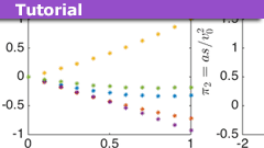
This relationship is illustrated in the following figure:

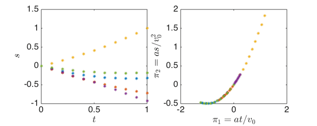
Left: Displacement $s$ as a function of $t$ for randomly chosen $v_0$ and $a$ (arbitrary units). There is no clear and easily identifiable relationship. Right: The same data but with $s$ and $t$ replaced by the dimensionless quantities $\pi_2$ and $\pi_1$. The physical relationship is clear and given by $\pi_2 = \pi_1 + \pi_1^2/2$.

---

I hope you enjoyed the read. If interested, you can read a bit more about dimensional analysis and modeling and reporting results using dimensional analysis in my book.

Comment Thread