P vs. NP and what is a Turing Machine (TM)?

P or NP

This article deals with the complexity of calculations and in particular the meaning of

$P\stackrel{?}{\neq}NP$

Before we explain what P and NP actually are, we have to solve a far bigger problem: What is a calculation? And how do we measure its complexity? Many people might answer, that a calculation is an algebraic expression and its complexity is the number of additions, subtractions, multiplications, and divisions. However, isn’t a division more complex than an addition? Isn’t it strange, that we did not use the words problem or result? And what if we decided to differentiate or integrate? It becomes clear that we need better tools and a preciser language if we want to make all these terms rigorous. The task is clear

 Problem  $\;\longrightarrow \;$  Computer $\;\longrightarrow \;$ Result

We need an alphabet to write the problem, a computer to do the calculations, and a decision whether we achieved a result or not. Everybody who ever mistakenly wrote an endless loop knows that the last part is not trivial. Let’s start with an example with true and false. This should easily fit into our scenario.

SAT

Let $\{x_1,\ldots,x_n\}$ be a set of Boolean variables. $L=\{x_1,\ldots,x_n,\bar{x}_1,\ldots,\bar{x}_n\}$ where $\bar{x}$ is interpreted as the negation of $x$ is called a set of literals. Any subset of $L$ is called a clause. A function

$f\, : \,L \longrightarrow \{\text{ true } , \text{ false }\}$

is called a consistent setting if $\bar{x}_k=1\oplus x_k$ for all $k.$ We call a set of clauses $C=\{C_1,\ldots,C_m\}$ satisfiable if there is a consistent setting such that every clause contains at least one true. We have OR’s within the clauses and AND’s between them. E.g. $\{\{x_1,x_2\},\{x_1,\bar{x}_2\},\{\bar{x}_1,x_3\},\{\bar{x}_1,\bar{x}_3\}\}$ is not satisfiable, $\{\{x_1,x_2\},\{\bar{x}_1,\bar{x}_2\}\}$ is satisfiable by $f(x_1)=\text{true}$ and $f(x_2)=\text{false}.$ The general problem

Given a finite set of clauses, decide whether it is satisfiable.

is called boolean satisfiability problem, SAT for short. If we restrict all allowed clauses to maximal $k$ literals, then we speak of $k$-SAT. Both examples above are in $2$-SAT. It can be shown that SAT and $3$-SAT is equivalent with respect to a polynomial computation complexity, i.e. in particular with respect to the computation classes $P$ and $NP.$

This is a famous example of a problem and its result $C=C_1\wedge C_2\wedge \,\ldots\,\wedge C_m.$ We have found a consistent setting in case $C=\text{true}$ which means the problem is satisfiable, and if there is no consistent setting, then $C=\text{false}$ for all settings and the problem is unsatisfiable. It remains to define the computer.

Register Machine (Computer)

A register machine consists of a finite, numbered set of registers that can be filled with any non-negative integer. The content of the registers can be changed, determined by the machine language. A program can (a) add one to a register, (b) subtract one from a register with positive content, (c) iterate those steps, (d) loop while a register’s content is positive.

A register machine is a rather primitive computer, but if you think about it, not much different from a real computer that has only RAM as available memory. We need OR, AND, and NOT for our satisfiability problem. But these logical operators can be computed with boolean, hence binary addition and multiplication:
\begin{align*}
x\text{ OR }y &= x\,\oplus\,y\,\oplus\,x \otimes y\\
x\text{ AND }y &=x \otimes y\\
\text{ NOT } x&= 1\oplus x
\end{align*}
so a register machine can handle SAT.

Turing Machine, 1936

Alan Turing (1912-1954) proposed a mathematical model of a computer back in 1936, long before the construction of the first electronic, programmable devices (Zuse 1938, 1941). His model mainly consisted of a computation tape, infinite at both ends, and linearly structured by cells that each can be filled with a single sign from a finite alphabet $a_0,\ldots,a_r.$ In addition, there is a controller instance that performs a read or write operation on a (working) cell or a shift to the next cell to the left or to the right.

 

 

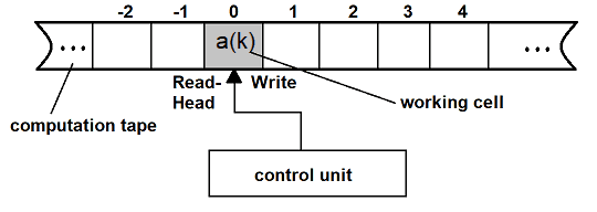
Besides “print $a(k)=a_k$” on the working cell, shift left, and shift right, we also allow “begin … end”, “while … repeat …” and “if … then …” as programmable steps. The computation of a Turing machine is a finite or infinite sequence of changing its configuration. A Turing machine accepts a starting configuration if it leads to an accepted final configuration, otherwise, it rejects the starting configuration. If the computation is infinite, then a starting configuration is neither accepted nor rejected. Long story short: A Turing machine solves a problem, i.e. a given starting configuration if it stops in a predefined final configuration after finitely many steps.

For our SAT problem, this means whether the starting configuration “all possible settings of literals” will stop at $\text{true}$ or $\text{false}$ in the final configuration. Since we can test all possible settings by brute force, our algorithm will certainly stop after finitely many steps with one or the other result. A Turing machine is, other than a registry machine, quite different from a real computer. However, it has the advantage that configurations and programming are nicer to handle than arbitrary non-negative integers in arbitrary many registers. We have only one location where changes over a finite alphabet happen. Most remarkable is that we get a natural definition of complexity, namely the number of changes of configurations of the tape during a computation, an algorithm that stops. So what have we lost? Nothing!

Theorem: Every program on a registry machine can be simulated by a program on a Turing machine over the alphabet $\{\text{blank}, 0, 1\}.$

A deterministic Turing machine is formally a $7$-tuple
\begin{align*}TM=(Q,\Sigma ,\Gamma ,\delta ,q_{0},a_0=\text{blank} ,F)\end{align*}

with a finite set $Q$ of possible configurations, $\Sigma$ a finite input alphabet, $\Gamma =\{a_0,\ldots ,a_r\}\supseteq \Sigma$ a finite tape alphabet, $F\subseteq Q$ the set of accepted final configurations, $q_0\in Q$ the starting, initial configuration, and a transition function
\begin{align*}\delta\, : \,(Q\setminus F)\times \Gamma \to Q\times \Gamma \times \{\text{ left },\text{ no move },\text{ right }\}.\end{align*}

An algorithm is a sequence $A=(q_0,q_1,q_2,\ldots) \subseteq \mathbb{P}(Q)$ where $(q_{i+1},a_{j(i+1)},*)=\delta(q_i,a_{j(i)}).$ We say that the TM stops on $q_0$ if there is a finite algorithm $(q_0,q_1,q_2,\ldots,q_m\in F)$ that ends in an accepted final configuration. Its length $m$ is called the runtime of $A,$ the number by the read-write-head inspected cells on the tape is called the space requirement of $A.$

Computation Class P

We restrict ourselves to decidability problems in order to define computation classes, i.e. problems with a binary result or final configuration true or false. The theorem allows us to concentrate on problems for Turing machines and algorithms that come to a hold on them. 3-SAT is such a problem. But deciding satisfiability for 2 clauses is certainly easier than for 2,000 clauses. The length of the input for our algorithm comes into play at this point. An input of 2 clauses is probably shorter than one with 2,000 clauses.

A set $D$ of problems is contained in the class P of in polynomial runtime decidable problems if there exists a Turing machine and a real polynomial $T(X)\in \mathbb{R}[X]$, such that every instance $I\in D$ of binary length $n$ can be decided by an algorithm of runtime $T(n).$

It is basically an algorithm that comes to an end after $O(n^\gamma)$ many steps with a constant $\gamma.$ E.g. let us consider matrix multiplication of $n \times n$ matrices
$$(a_{ij})\cdot (b_{kl}) = \left(\sum_{r}a_{pr}b_{rq}\right).$$
We have $n^3$ multiplications and additions. Hence matrix multiplication belongs to the computation class $P$ for polynomial runtime. V. Strassen has shown 1969 that it can be done in $O(n^{2.807})$ at the expense of more additions.

We have seen that the brute force method of checking a $3$-SAT problem needs $O(2^n)$ steps where $n$ is the number of literals. This is an exponential runtime and no more polynomial. Hence $3$-SAT cannot be solved within $P$ by brute force. It does not say, that there isn’t another polynomial runtime algorithm that does the job. Well, let’s be honest, we don’t know any. However, if we could ask an oracle for a consistent setting, then we can easily check in polynomial (actually constant) runtime whether this single solution is true or false.

Computation Class NP

This leads us to the computation class NP. The letters stand for non-deterministic polynomial runtime. The polynomial part is easily explained. It means that we can verify a solution in polynomial time, just as a consistent setting for $3$-SAT. But what does non-deterministic mean?

A deterministic Turing machine has a transition function that determines three variables given a configuration and a letter in the working cell: the letter that has to be written into the working cell, whether and which direction the read-write-head has to be moved, and the configuration that has to be changed into. A non-deterministic Turing machine has a transition function that does not uniquely determine these three variables anymore. There are several possible transitions. Hence a non-deterministic Turing machine doesn’t have one predetermined execution but rather has many possible ones. This can be interpreted that it randomly chooses one out of the many executions, or that it executes all possible ones in parallel. A non-deterministic Turing machine accepts input if there is an allowed execution for it. The picture of parallel execution is the reason for the rule of thumb:\begin{align*}P\, &: \,\text{ polynomial runtime }\\NP\, &: \,\text{ exponential runtime }\end{align*}

But please do not take this too seriously. NP still requires a polynomial runtime verification.

A set $D$ of problems is contained in the class NP of in polynomial runtime non-deterministic decidable problems if there exists a non-deterministic Turing machine and a real polynomial $T(X)\in \mathbb{R}[X]$, such that for every instance $I\in D$ of binary length $n$ holds:

If the answer to $I$ is true, then there is an algorithm of runtime $T(n)$ such that the non-deterministic Turing machine stops in the final state true.

If the answer to $I$ is false, then the non-deterministic Turing machine either never stops on any algorithm of length $T(n)$, or in the state false.

$3$-SAT can be verified in polynomial time, and if we imagine that all $2^n$ inputs could be tested in parallel, we would certainly get the decision whether there is a consistent setting or not, too, in polynomial time. Hence $3$-SAT is an NP-problem.

Every deterministic Turing machine is also a non-deterministic Turing machine, even if all possible executions of an algorithm boil down to one, i.e. \begin{align*}P\subseteq NP.\end{align*}

Whether equality holds is the $P=NP$ or more likely $P\neq NP$ conjecture.

“Because quantum computers use quantum bits, which can be in superpositions of states, rather than conventional bits, there is sometimes a misconception that quantum computers are non-deterministic Turing machines. However, it is believed by experts (but has not been proven) that the power of quantum computers is, in fact, incomparable to that of non-deterministic Turing machines; that is, problems likely exist that a non-deterministic Turing machine could efficiently solve that a quantum computer cannot and vice versa.” [4],[5]

There is also a computation class co-NP. It contains the complement to NP, i.e. all decidability problems for which we have an algorithm that decides in polynomial time on a non-deterministic Turing machine that a certain instance does not represent a solution to a problem. It is basically an exchange of true and false in the formal definition above. $\text{P}\subseteq \text{NP}\cap \text{co-NP},$ however, it is unknown whether $\text{NP}\stackrel{?}{=}\text{co-NP}.$

NP-completeness

A decidability problem $E$ is said to be NP-complete, if for any problem $D\in NP$ there is a function $f\, : \,D\rightarrow E$ that can be computed in polynomial time in the binary input length of $D$, such that every algorithm that decides $E$ also decides $D$ at an extra cost of polynomial time. If we drop the requirement $D\in NP,$ i.e. consider arbitrary decidability problems, then we speak of NP-hard problems.

NP-complete problems have therefore sort of maximal complexity within NP or may be called universal for their computation class.

 

Theorem: Let $E$ be a NP-complete problem. Then

\begin{align*}E\in P \Longleftrightarrow P=NP.\end{align*}

Steven Cook has shown 1971, and independently Leonid Levin 1973, that SAT is NP-complete. So everybody who could solve $3$-SAT in polynomial time would also prove $P=NP.$ Cook particularly solved the question of whether there are NP-complete problems at all!

We meanwhile know many NP-complete problems. An (incomplete) list can be found in [6]. The most famous ones are probably SAT, Knapsack (how to load a truck), and traveling salesman (find the shortest way to all customers). We see that NP-complete problems are not just a theoretical playground, their solutions have monetary value! Have you ever wondered how airlines staff their flights? Or how trains are scheduled? There were rumors that Strassen’s improvement of matrix multiplications [7] found its way into airliner cockpits! Note, that we wrote 1969 when he reduced the matrix exponent from $3$ to $2.807$. What is no rumor, Strassen lost a bet that $P=NP$ would have been decided before the nineteenth century ended. I think the actual year was 1998 but I’m not sure I remember it correctly. He lost a trip over the Alps in a balloon.

Chances that P=NP

Manindra Agrawal, Neeraj Kayal, and Nitin Saxena published an algorithm in 2002 that decides whether an integer is prime or not in polynomial time without using conjectures like the Riemann hypothesis. Hence the prime number problem is in P. The sieve of Eratosthenes is not in P. This doesn’t tell us yet how hard the factorization problem is. We currently only know that it is in NP, but not if it is NP-complete or even in P.

The P vs. NP question has a philosophical dimension, too. We know a lot of problems, many of which are even real-world problems, that are in NP. Now, are they really intrinsically hard, or are we just too dumb to solve them with a smart polynomial runtime algorithm? The underlying assumption is that polynomial runtime is doable, whereas NP-hard problems require exponential runtime, and are thus not doable as soon as the input length is of any interest. This is more of a philosophical rather than a practical question. Sure, polynomial runtime algorithms are faster than exponential runtime algorithms, and in particular, easier to improve further. However, this is only true as long as the polynomials are of small degrees. An NP-complete problem which we could solve in $O(n^{(10^{1000})}))$ steps would still require a very, very big machine to actually execute it. It would prove $P=NP$ but would be of little help to load a truck. So far, only exponential runtime algorithms on deterministic computing machines are known for solving NP-complete problems exactly. However, it is not proven that there are no polynomial runtime algorithms for the solution, in contrast to another class of problems that are guaranteed to take at least exponential running time and are thus provable outside P.

Most scientists believe that $P\neq NP,$ i.e. that there are really hard problems that cannot be solved deterministically in polynomial runtime. However, until 2002, many scientists might have thought that PRIME is not in P, too, or only if the extended Riemann hypothesis holds.

The question P versus NP made it on the list of the millennium prize problems of the Clay Mathematics Institute in 2000. [9]