Posterior Predictive Distributions in Bayesian Statistics

Confessions of a moderate Bayesian, part 4

Bayesian statistics by and for non-statisticians

Read part 1: How to Get Started with Bayesian Statistics

Read part 2: Frequentist Probability vs Bayesian Probability

Read part 3: How Bayesian Inference Works in the Context of Science

Predictive distributions

A predictive distribution is a distribution that we expect for future observations. In other words, instead of describing the mean or the standard deviation of the data we already have, it describes unobserved data.

Predictive distributions are not unique to Bayesian statistics, but one huge advantage of Bayesian statistics is that the Bayesian posterior predictive distribution considers the uncertainty of the parameters. This makes the Bayesian posterior predictive distribution a better representation of our best understanding of the process that generated the data.

Basic concept

One of the core ideas of statistics is to make a model of the data generating process. Usually, this model has some unknown parameters that are estimated from the data itself. Often those parameters tell us something important about the system, so often we are just interested in the parameters. But, once we have those parameters, we can turn around and use the model with the parameters to predict what we would expect as new observations.

In Bayesian statistics, we don’t end up with point estimates of the parameters but samples of the posterior joint distribution of the parameters. To get samples of the posterior predictive distribution we take a sample from the posterior parameter distribution, get a set of parameters, plug those parameters into the model, and generate a predicted sample of the data. The distribution of those predictions is the posterior predictive distribution.

Uses

The main use of the posterior predictive distribution is to check if the model is a reasonable model for the data. We do this by essentially simulating multiple replications of the entire experiment. For each data point in our data, we take all the independent variables, take a sample of the posterior parameter distribution, and use those to generate a sample of posterior predictive distribution of the data. We can repeat this multiple times, generating multiple complete replications of the exact same experiment. If our simulated data looks like our actual data, then the model is reasonable.

Another use of the posterior predictive distribution is to see what we would expect to change because of some proposed intervention. In this case, we follow a process like what we described above, except that instead of using the independent variables as specified in the actual experiment we modify the independent variables to reflect our proposed intervention. Then we can simulate what difference that change would make compared to the original data or compared to a different intervention.

Checking model quality

First, I will show how to use the posterior predictive distribution to check and refine the model.

Chicken growth models

In a previous Insights I used the “chickweights” data set. I now return to that data set. This data set examines the growth (weight) of a large number of baby chickens from hatching to 21 days. The chicks are split into four groups which were fed different diets.

Generating the posterior predictive distribution

First, we load some necessary libraries and the data itself. And as before we will exclude the data from less than one week of age.

library(rstanarm)
library(ggplot2)
library(bayesplot)
library(emmeans)
data("ChickWeight")
dat <- subset(ChickWeight,Time > 7)

Next, we will specify our model and sample the posterior distribution of the model parameters. In this case we will model the weight of each chick as being normally distributed with a mean that depends linearly on the age of the chick (Time) and on the feed being used (Diet) for that chick.

set.seed(4567)
post <- stan_lm( weight ~ Diet*Time, data = dat, prior = R2(.7))

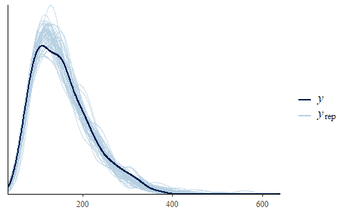
Once we have the posterior distribution of the model parameters then we can generate the posterior predictive distribution of the data. In this case, we will generate 500 predicted replicates of the original experiment. We will then plot the probability density function (PDF). We will display the PDF of the original data together with the PDF of the first 50 predicted replicates to see how well they match.

w <- dat$weight
wrep <- posterior_predict(post,draws = 500)
ppc_dens_overlay(w, wrep[1:50,])

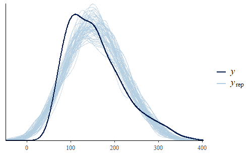
As we can see, the posterior predicted distribution does not match the actual data very well. So let’s dig a little deeper and see if we can find the cause of this discrepancy.

Examining model discrepancies

First we will do a scatter plot of the average of the posterior predicted data vs the original data. This will help us look for patterns of deviations in our predictions vs the data.

ppc_scatter_avg(w, wrep)

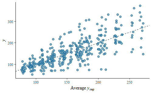
The simulated data looks pretty good overall, there is no systematic departure from the identity line. However, we do notice that the variance is substantially smaller for lower weights than for higher weights. We can explore this further by calculating some summary statistics on the predicted replicates and compare that to the same summary statistic calculated on the original data. We will calculate the mean and the min of the data and each replicate.

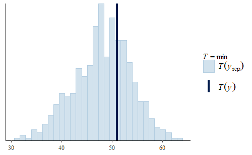
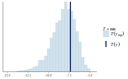
ppc_stat(w, wrep, stat = "mean")
ppc_stat(w, wrep, stat = "min")

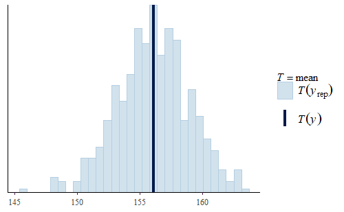
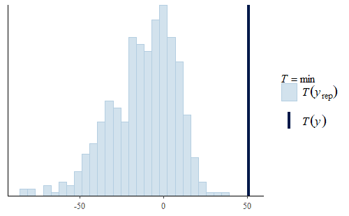
Here, we see two interesting facts.

First, the mean is quite good. The actual mean of the original data is very representative of the means of the replicates. This is quite common since the mean was specifically modeled. So the model will accurately represent the mean of the data even though the model does not capture other features of the data. If all you wanted to do was make inferences about the mean, then you could in fact use this model as it is. This is an important point, a model is not just “good” or “bad”, but the value of a model depends on what it will be used for.

Second, the min is not very good. The actual min of the original data is well above the range of the mins of the replicates. In fact, the minimum weight in the original data is about 50 g, but the model usually has negative minimum weights. Not only is that a strong discrepancy with the data, negative weights don’t make any physical sense either.

Improving the model

Luckily, we can make one single change that will address both the increasing variance with larger predictions and also the negative weights. Instead of modeling the weights themselves as normally distributed, we will model the log of the weights as normally distributed.

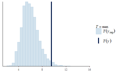
post <- stan_lm( log(weight) ~ Diet * Time, data = dat, prior = R2(.7))
w <- dat$weight
wrep <- exp(posterior_predict(post,draws = 500))
ppc_dens_overlay(w, wrep[1:50,])
ppc_stat(w, wrep, stat = "min")

This time we see that the PDF of the posterior predictive distribution closely matches the PDF of the original data. Furthermore, the min is much more reasonable, with a smaller range that includes no negative weights and the actual data min is very representative of the mins of the replicates.

Using the model for custom information

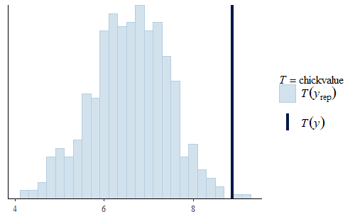
At this point, we now feel confident in using our model to make predictions about the min as well as the mean. But having found a model which seems to capture the data faithfully we can now turn to look at features that might be of more direct interest. For example, suppose that our customers purchase chicks by weight at 21 days, but will not accept any chicks less than 150 g. Then our main interest might be the total weight (in kg) of all birds over 150 g at day 21 which would be (proportional to) the value of the chicks.

chickvalue <- function(x){
   return(sum((dat$Time == 21)*(x>150)*(x)/1000))
}
ppc_stat(w, wrep, stat = "chickvalue")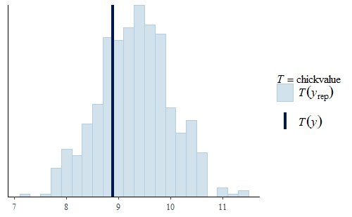

Here we see that even though the model was not specifically fit to the “chickvalue” measure, because it is a faithful representation of the data overall, the model seems to be suitable to represent this aspect of the data as well.

Note that the model still has limitations. For example, even though the data contains information about the number of chicks that died during the 21 days, we did not model that. So if we look at our replicate data sets we will find that they all have the exact same rate of chick survival

livechick <- function(x){
   return(sum(dat$Time == 21)/sum(dat$Time == 8))
}
ppc_stat(w, wrep, stat = "livechick", binwidth = .01) + coord_cartesian(xlim = c(.70, 1))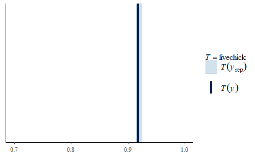

Heteroskedastic data

Shifting gears, I will now discuss a data set that came up in some research at work recently. It consists of six different measurement techniques (all measuring the same quantity) on several samples of standards with known values of the measured quantity. Because the samples have known values we could determine the error of each measurement. We were attempting to characterize the bias and precision of the six techniques.

After playing around with different models for more than a full day at work the best model that I could find was the following

set.seed(4567)
post <- stan_lmer(Err ~ Correction|Segment, data = dat.pdff,
          diagnostic_file = file.path(tempdir(), "post.csv"), contrasts = FALSE, adapt_delta = 0.999)

y <- dat.pdff$Err
yrep <- posterior_predict(post,draws = 500)
ppc_dens_overlay(y, yrep[1:50,])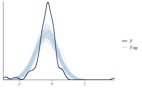

As you can see, the PDF of the replicates is clearly different from the PDF of the original data. We see that the interquartile range of the model is too large and yet the model’s min and max are both not extreme enough. The model has a fairly standard Gaussian shape while the data has a sharp peak and heavy tails.

Upon further investigation, it became clear that the issue was some strong heteroskedacity of the data. Specifically, although all the methods seemed to have similar small bias, two of the methods were substantially less precise than the others.

ggplot(dat.pdff,aes(x=Correction,y=Err)) +
  geom_boxplot(outlier.shape = NA) +
  geom_jitter(aes(color = Segment), alpha = 0.5)

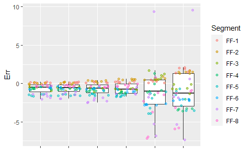
This is an issue that comes up frequently in real data where the variances are not equal. However, most statistical methods assume that the variance is equal across the data. This is such a standard assumption that many researchers forget about it entirely. However, Bayesian analysis can go beyond this limitation and we can directly model the heteroskedasity. So I ran a new analysis, this time modeling the errors as being normally distributed with a mean and a standard deviation that both depend on the measurement technique.

post <- brm(bf(Err ~ Correction, sigma ~ Correction), data = dat.pdff, family = gaussian())
y <- dat.pdff$Err
yrep <- posterior_predict(post,draws = 500)
ppc_dens_overlay(y, yrep[1:50,])
ppc_stat(y, yrep, stat = "median")
ppc_stat(y, yrep, stat = "min")
ppc_stat(y, yrep, stat = "max")

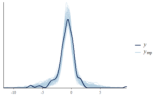
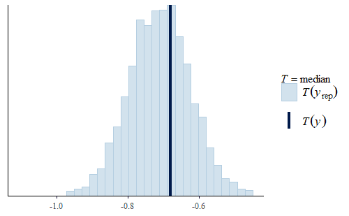
This time the PDF of the actual data is representative of the PDF of the posterior predicted replicates. The IQR, min, and max are also all reasonably well represented.

Interestingly, the max of the data is somewhat on the high side of the range of maxes of the replicates. The max of the data is basically a single data point that appears to be a bit of an outlier. I do not reject data simply because it seems like an outlier, and since I did not have any experimental reason for rejecting that data point we retained it in the analysis.

I did not do any manual “tweaking” or other games to reduce the impact of that data point. But the Bayesian method itself automatically included a bit of healthy skepticism about that data point. It chose a model where that point is not implausible, but it also chose a model where we do not expect quite such an extreme outlier in most of our predicted replicates. If I were going to do some manual “tweaking” of the model, that is exactly what I would have chosen: a model which is informed by the possible outlier but not entirely beholden to it.

Investigating treatment predictions

By far, most of my experience with posterior predictive distributions has centered around the use case of critiquing and refining the model. However, the posterior predictive distribution is so named because you can use it to make predictions. Instead of making a prediction based on the actual experiment, you can make predictions based on hypothetical data using the model developed from the actual data.

For example, let’s return to the ChickWeights data. Now we have a good model that looks like it plausibly captures the main features of the data.  In particular, we think that the model does a good job representing how much chicken we expect to be able to sell (total weight of all chicks larger than 150 g at 21 days). So now, let’s do two simulations, one where we simulate feeding all the chicks with diet 3 and another where we simulate feeding all the chicks with diet 1. To generate the data for simulation we do the following:

dat.diet3 <- dat
dat.diet3$Diet[] <- 3
dat.diet1 <- dat
dat.diet1$Diet[] <- 1

Then we generate and plot the posterior predictions using the following code:

w <- dat$weight
wrep <- exp(posterior_predict(post, draws = 500, newdata = dat.diet1))
ppc_stat(w, wrep, stat = "chickvalue", binwidth = 1)
wrep <- exp(posterior_predict(post, draws = 500, newdata = dat.diet3))
ppc_stat(w, wrep, stat = "chickvalue", binwidth = 1)

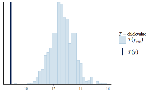
So based on this posterior prediction, we would expect that if we were to use exclusively Diet 1 then we would get around 7 kg of sellable birds for this size batch. In contrast, for Diet 3 we would expect around 13 kg of sellable birds. That is a substantial difference. Based on this model and the experiment, we could compare the costs of raising the chicks to 21 days using the two different diets and thus determine which is the more profitable approach. And note that this approach completely avoids any inappropriate overemphasis on whether the difference is “statistically significant”.

Summary

I am still new to using posterior predictive distributions, but they have already become my favorite tool for examining, criticizing, and improving a model. Using arbitrary statistics that are individually tailored to a specific need is intriguing to me. And I especially like this tool for checking the appropriateness of the model for any statistic.

I also have found that sometimes model parameters themselves can become difficult to interpret. I have occasionally avoided a specific model, not because I had any valid statistical or experimental reason to do so, but because the parameters were too confusing to interpret. The posterior predictive distribution can help with that by focusing attention on the predicted hypothetical observations, especially since the observations usually represent a quantity that is of direct interest to the researchers. Overall, I have found the posterior predictive distribution to be an exceptionally useful and flexible tool.

Comment Thread