The Quantum Liar Experiment: An Instantiation of the Mermin Device

In 1981, Mermin published a paper[1], “Bringing home the atomic world: Quantum mysteries for anybody” in which he explained the mystery of quantum nonlocality[2] without requiring the formalism of quantum mechanics (QM). I will summarize that argument then show how the QM formalism fits his results and how his device is instantiated in Elitzur & Dolev’s quantum liar experiment (QLE)[3]. The quantum state of the Mermin device and the QLE can be created and tested in the undergraduate physics laboratory[4], so while the Mermin device and the QLE are hypothetical, no one doubts their QM predictions.

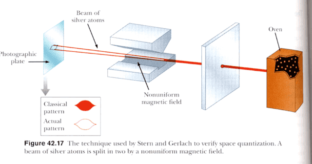
The Mermin device is shown in his Figure 2 below. Two particles are emitted from the Source C towards the two detectors A and B. Let the experimentalist controlling detector A be Alice and the experimentalist controlling detector B be Bob. Alice and Bob may choose one of three settings (labeled 1, 2, or 3) for their detector on each run of the experiment. This decision can be made at any time before the particle reaches the detector. There are two possible outcomes for any given setting, red (R) and green (G). As we will see later, these settings can correspond to polarizer settings for photons or Stern-Gerlach (SG) magnet orientations for spin measurements (Serway & Jewitt Figure 42.17 below). The two outcomes correspond to pass or no pass for the polarizer and spin up or spin down for the SG magnet. But, you don’t have to do any QM calculations to understand the mystery as Mermin explains it. Let’s look at his simple explanation.

Many trials of the experiment are performed with Alice and Bob changing their detector settings randomly while the particles traverse the space between the Source and detectors, so Alice chooses setting 1 as often as setting 2 as often as setting 3 and Bob does the same. Here are the results:

1. Alice finds 50% R and 50% G outcomes for each detector setting 1, 2, and 3, regardless of what Bob did. Bob finds the same regardless of what Alice did.
2. In 25% of the trials, Alice and Bob both measured G, regardless of their detector settings.
3. In 25% of the trials, Alice and Bob both measured R, regardless of their detector settings.
4. When the settings are the same, i.e., 11, 22, or 33, the outcomes are always the same, i.e., RR or GG (occurring with equal frequency).

Results 1-3 can be explained if the particles are emitted with random distributions of color for each possible setting. Thus, there is a 50% probability of measuring R for any given setting in each trial and a 50% probability of measuring G for any given setting in each trial for both Alice and Bob (result 1). That means the possible correlated outcomes RR, GG, RG, and GR occur with equal frequency, regardless of detector settings, which explains the 25% GG and 25% RR outcomes (results 2 and 3, respectively). However, result 4 makes things difficult to explain.

As I pointed out in a previous Insight with Mermin’s explanation of the Hardy experiment, the particles don’t ‘know’ how they will be measured in any given run, in fact the detector settings can be chosen an instant before the particles arrive at their respective detectors. And, assuming the measurements are space-like separated, no information about the setting and outcome at one detector can reach the other detector before the particle is measured there, i.e., the measurements are said to be “local.” Thus, the particles don’t know how they will be measured when they are emitted and they can’t transmit that information to each other during the run. So, it seems the particles’ possible outcomes with respect to each possible detector setting must be coordinated to guarantee the like outcomes GG and RR for like settings 11, 22, or 33. Mermin calls the coordination of outcomes “instruction sets” and the fact that the particles have definite properties corresponding to possible measurements whether they are carried out or not is called “realism” or “counterfactual definiteness.” The combination of these assumptions is often called “local realism” or “Einsteinian local realism”[5]. Both assumptions seem reasonable, locality because the temporal order of space-like separated events is frame dependent according to special relativity, which would seem to rule out superluminal information transfer, and realism because the particles don’t ‘know’ how they will be measured until the last moment and they have to guarantee like outcomes for like settings. So, let’s look at all the runs where the particles are both emitted with the instruction set 1G2G3R, for example.

There are nine possible setting combinations: 11, 22, 33, 12, 13, 23, 21, 31, 32. We’re guaranteed to get like outcomes in settings 11 (GG), 22 (GG) and 33 (RR), by design. But, we also get like outcomes in settings 12 (GG) and 21 (GG). That means we get like outcomes in 5/9 of the trials. Any instruction set other than 1G2G3G or 1R2R3R will give this 5/9 agreement and the exceptions give 9/9 agreement, so the overall expected agreement is greater than 5/9. This is called a “Bell inequality” and our QM results 2 and 3 above violate this inequality, since we only have agreement in half the trials. Mermin challenges the reader to find a locally realistic way to make results 1-4 above obtain and 35 years later that challenge has not been met (although those in the retrocausality program would disagree!). Retrocausality aside, it seems to be the case that counterfactual definiteness (instruction sets) does not obtain. Now let’s look at the QM formalism behind this result.

I’ll do this with spin, since that’s the premise for the QLE, but the QM state I’m using here has been created with photons and shown to violate the Clauser-Horne-Shimony-Holt version of the Bell inequality[4]. Spin is a quantum property as shown in Serway & Jewitt’s Figure 42.17 below. Let the orientation of the SG magnet in Figure 42.17 be called the Z direction. If the atom is deflected towards the north magnetic pole it’s said to have “spin up” (Z+) and if it’s deflected towards the south magnetic pole, it’s said to have “spin down” (Z-). Let spin up correspond to a G outcome and spin down an R outcome in the Mermin device. The Source in the Mermin device emits a pair of atoms in the Z spin state

\begin{equation} \mid \Psi \rangle = \frac{1}{\sqrt{2}}\left(\mid ++ \rangle + \mid -\:- \rangle \right) \label{state1} \end{equation}

where the first “+” in $\mid ++ \rangle$ refers to atom 1 at detector A and the second “+” refers to atom 2 at detector B. Likewise with “-“. The probability of measuring a ++ outcome is given by $\mid \langle ++ \mid \Psi \rangle \mid ^2 = \frac{1}{2}$ since $\langle ++ \mid ++ \rangle = 1$ and $\langle ++ \mid -\:- \rangle = 0$. Likewise, the probability of measuring a – – outcome is $\mid \langle -\:- \mid \Psi \rangle \mid ^2 = \frac{1}{2}$. The outcomes + – and – + are not possible in this state, i.e., if Alice and Bob both measure Z, they will never get different results. If we decide to rotate our SG magnets by an angle $2\theta$, the individual components of $\Psi$ rotate by $\theta$, i.e.,

\begin{equation} \mid ++ \rangle = \left(cos\left(\theta\right) \mid \tilde{+}\rangle – sin(\theta)\mid \tilde{-}\rangle\right)\left(cos\left(\theta\right) \mid \tilde{+}\rangle – sin(\theta)\mid \tilde{-}\rangle\right) \label{state2} \end{equation}

Likewise

\begin{equation} \mid -\:- \rangle = \left(sin(\theta) \mid \tilde{+}\rangle + cos(\theta)\mid \tilde{-}\rangle\right)\left(sin(\theta) \mid \tilde{+}\rangle + cos(\theta)\mid \tilde{-}\rangle\right) \label{state3} \end{equation}

(see Figure 1c). Adding Eqs(\ref{state2} & \ref{state3}) we get

\begin{equation} \mid ++ \rangle + \mid -\:- \rangle = \mid \tilde{+}\tilde{+}\rangle + \mid \tilde{-}\:\tilde{-}\rangle \label{state4} \end{equation}

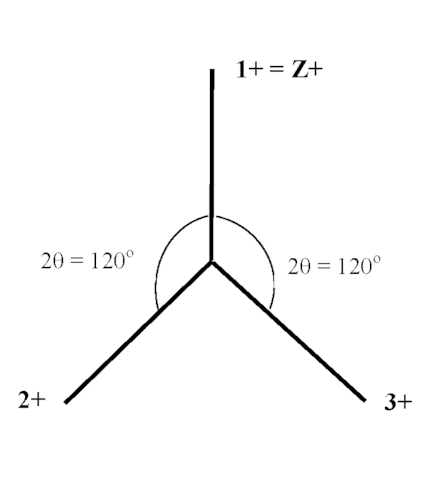
Thus, everything I said about the probabilities with respect to the Z direction is true for any orientation of the SG magnets. We will restrict the possible orientations of the two SG magnets of the Mermin device to the Z direction (which I will call the “1” direction) and $120^o$ with respect thereto (Figure 1f). Thus, we see how the QM formalism maps to results 1 and 4. In order to see how it maps to results 2 and 3, we need to find the probability of like results in unlike settings, i.e., we need to compute $\mid \langle \tilde{+}+ \mid \frac{1}{\sqrt{2}}\left(\mid ++ \rangle + \mid -\:- \rangle \right)\mid ^2$ and $\mid \langle \tilde{-}\: – \mid \frac{1}{\sqrt{2}}\left(\mid ++ \rangle + \mid -\:- \rangle \right)\mid ^2$. Both give the same result, i.e.,

\begin{equation} \mid \langle \tilde{+}+ \mid \frac{1}{\sqrt{2}}\left(\mid ++ \rangle + \mid -\:- \rangle \right)\mid ^2 = \frac{1}{2}\left(\langle \tilde{+}+ \mid ++ \rangle + \langle \tilde{+}+ \mid -\: – \rangle \right)^2 = \frac{1}{2}\left(\langle \tilde{+}\mid +\rangle \langle + \mid + \rangle + \langle \tilde{+} \mid – \rangle \langle + \mid – \rangle \right)^2 = \frac{1}{2}\left(\langle \tilde{+}\mid +\rangle \right)^2 = \frac{1}{2} cos^2(\theta) \label{prob1} \end{equation}

since $\langle + \mid + \rangle = 1$ and $\langle + \mid – \rangle = 0$. With $\theta = 60^o$ Eq (\ref{prob1}) gives a probability of ++ outcomes in unlike settings ($\frac{2}{3}$ of all trials) of $\frac{1}{8}$. The probability of a ++ outcome in like settings ($\frac{1}{3}$ of all trials) is $\frac{1}{2}$ (as shown above), so the probability of a ++ outcome for the experiment overall is $\frac{1}{8} \frac{2}{3} + \frac{1}{2} \frac{1}{3} = \frac{1}{4}$, i.e., result 2. The same result holds for the probability of a – – outcome which is result 3. So, the QM formalism tells us we will see results 1-4 and experiments confirm these results. Thus, it appears counterfactual definiteness (Mermin’s instruction sets) must be abandoned and that leads to the quantum liar paradox of the QLE, which is essentially an instantiation of the Mermin device. Let’s look at that result.

Suppose we place an atom into one of two transparent boxes according to its Z spin without knowing which box it’s in. For example, we replace the photographic plate in Serway & Jewitt’s Figure 42.17 (below) with a pair of glass boxes and let the oven run until we’re pretty sure we have captured one and only one atom. Let the orientation of the SG magnet in Figure 42.17 be called the Z direction. Now put these boxes into a Mach-Zehnder interferometer (MZI) as shown in Figure 1d below. An MZI works as explained in my Insight on the quantum Cheshire Cat. All we have to do is add a factor of i to our photon amplitude wherever we have reflections through the MZI (Figure 1a). Thus, the amplitude at detector D1 in Figure 1a is

\begin{equation} \left(\frac{1}{\sqrt{2}} \right)\left(i\right)\left(i \frac{1}{\sqrt{2}}\right) +\left( i\frac{1}{\sqrt{2}}\right) \left(i\right) \left(\frac{1}{\sqrt{2}} \right) = \: – 1 \label{Fig1a1} \end{equation}

Reading from left to right in each pair of parentheses connecting the Source to detector D1 we have contributions from two paths: (transmission at the first 1-1 beam splitter)(reflection from mirror M)(reflection at the second 1-1 beam splitter) + (reflection at the first 1-1 beam splitter)(reflection from mirror M)(transmission at the second 1-1 beam splitter). The relative intensity at D1 is the square of this amplitude, i.e., 1. Using the same rules we find the amplitude at D2 is given by

\begin{equation} \left(\frac{1}{\sqrt{2}} \right)\left(i\right)\left(\frac{1}{\sqrt{2}}\right) +\left( i\frac{1}{\sqrt{2}}\right) \left(i\right) \left(i\frac{1}{\sqrt{2}} \right) = \: 0 \label{Fig1a2} \end{equation}

Thus, every photon emitted by the Source arrives at D1 in Figure 1a. Now suppose we block one of the arms of the MZI as in Figure 1b. In this configuration, there is no contribution to the amplitude at D1 from the lower path so the amplitude at D1 is now

\begin{equation} \left(\frac{1}{\sqrt{2}} \right)\left(i\right)\left(i \frac{1}{\sqrt{2}}\right) = \: – \frac{1}{2} \label{Fig1b1} \end{equation}

Likewise, there is no contribution to the amplitude at D2 from the lower path so the amplitude at D2 is now

\begin{equation} \left(\frac{1}{\sqrt{2}} \right)\left(i\right)\left(\frac{1}{\sqrt{2}}\right) = \: \frac{i}{2} \label{Fig1b2} \end{equation}

The amplitude at detector D3 is given by the signal in the lower half

\begin{equation} \left(i\frac{1}{\sqrt{2}} \right)\left(i\right) = \: -\frac{1}{\sqrt{2}} \label{Fig1b3} \end{equation}

So the intensity of the signal at each of detectors D1, D2, and D3 is $\frac{1}{4},\frac{1}{4}, \frac{1}{2}$, respectively.

Now return to the situation of Figure 1d and send a single photon through the MZI. If D2 clicks, we know the lower path is blocked because otherwise detector D1 will always click. However, since the photon reached D2 it didn’t go through the lower path of the MZI and interact with the atom there. But, since we know the lower arm is blocked we know the atom is in the Z+ box meaning we just did a spin Z measurement on our atom without interacting with it. Elitzur & Vaidman[6] call this “interaction-free measurement.” Now repeat this process with two pairs of boxes placed in the MZI per Figure 1e. If D2 clicks we know that one and only path of the MZI is open and the other is blocked, but we don’t know which path is open and which is blocked. Thus, we have created the state in Eq(\ref{state1}).

Suppose we repeat the construction of this state many times, passing the pair of glass boxes to Alice and Bob each time so they can perform spin measurements per the Mermin device (settings as in Figure 1f). Everything I said about this state above holds, so overall they each got 50% + and 50% -. Whenever they both did a measurement in the same setting, they both got + or they both got – (half ++ and half – -). Overall, they got ++ in 25% of the trials and they got – – in 25% of the trials. Everything holds so it must be the case that there are no instruction sets (no counterfactual definiteness), which means there aren’t any definite values of + or – in unmeasured settings. But what does that mean in a trial where, say, Alice did a measurement in setting 2 while Bob did a measurement in setting 3? Suppose Alice got – and Bob got +. We know that if Bob had done a setting 2 measurement he would’ve gotten – and had Alice done a setting 3 measurement she would’ve gotten +. That fixes the counterfactuals for settings 2 and 3, but what about setting 1? There can’t be any counterfactuals for setting 1 (Z measurement) because that would mean we have counterfactual definiteness (a complete instruction set) and we showed above that instruction sets don’t produce the right probabilities. But, wait a minute, don’t we also know that one and only one path was blocked in Figure 1e in order to get the state of Eq(\ref{state1}) which produced the outcomes in the first place? Having one and only one path blocked in Figure 1e definitely means 1+1+ or 1-1-, i.e., counterfactual definiteness for setting 1. It appears that in trials of this type we need counterfactual definiteness to produce the state that tells us there is no counterfactual definiteness. This is the quantum version of the liar paradox, e.g., “this sentence is a lie (false).” If the sentence is true, then it’s false. If it’s false, then it’s true. Thus, the name “quantum liar experiment” given by Elitzur & Dolev (who explain the QLE using an evolving blockworld[3]). [For other explanations of the QLE see Kastner[7] and Stuckey[8].] To see how the conundrum of the Mermin device can be resolved for the “general reader” who has taken introductory physics, see Quantum mysteries for anybody: Solved.

In the next Insight I will show how no counterfactual definiteness in the Greenberger-Horne-Zeilinger experiment as described by Mermin[9] and Dowker[10] is used to motivate Sorkin’s Many Histories interpretation of QM.

 

Figure 1a: Mach-Zehnder Interferometer

 

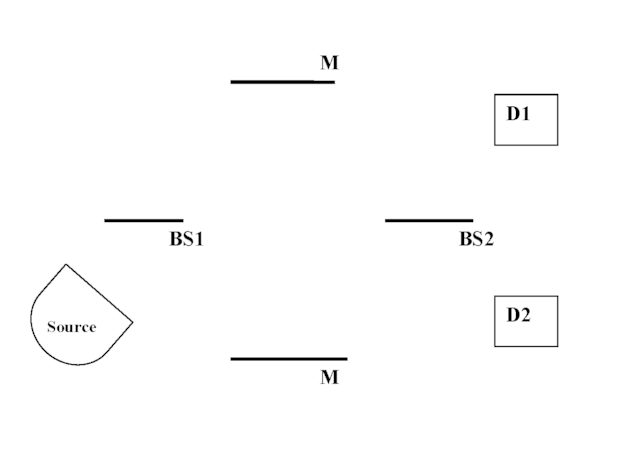
Figure 1b: MZI with One Path Blocked

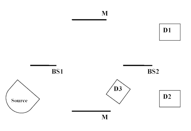
Figure 1c: Hilbert Space Rotation

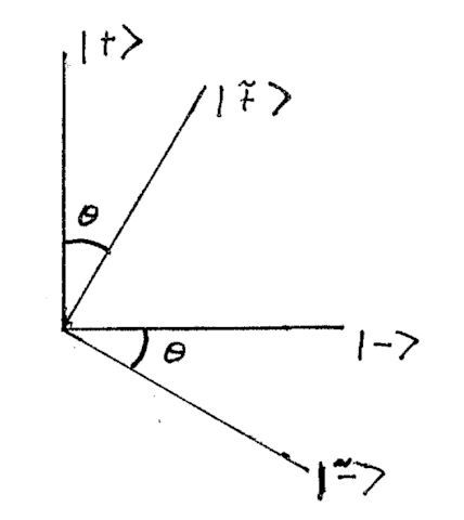
Figure 1d: Interaction-Free Measurement

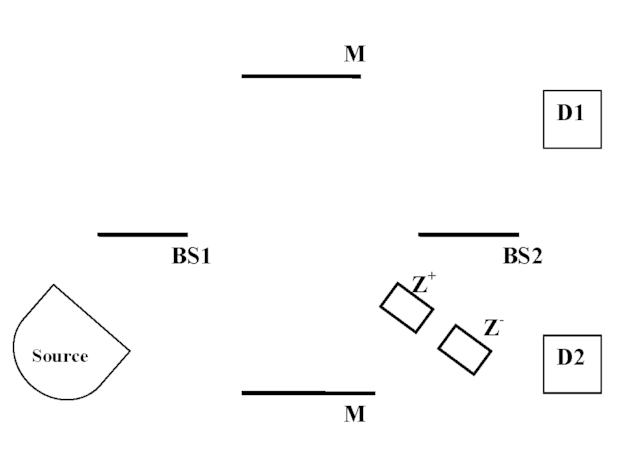
Figure 1e: Quantum Liar Experiment

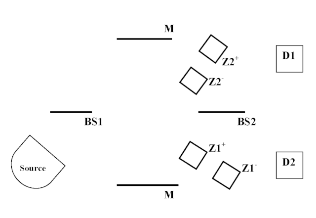
Figure 1f: Stern-Gerlach Magnet Orientations

 

 

Mermin Figure 2: The Mermin Device

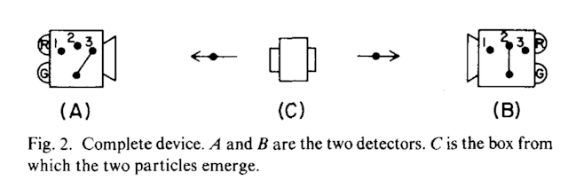
Figure 42.17 of Serway & Jewitt: Stern-Gerlach Magnet

 

Resources

1. Mermin, N.D.: Bringing home the atomic world: Quantum mysteries for anybody. American Journal of Physics 49, 940-943 (1981).
2. ““the phenomenon by which measurements made at a microscopic level contradict a collection of notions known as local realism that are regarded as intuitively true in classical mechanics” https://en.wikipedia.org/wiki/Quantum_nonlocality.
3. Elitzur, A., & Dolev, S.: Quantum Phenomena within a New Theory of Time: In: Elitzur, A., Dolev, S., & Kolenda, N. (eds.) Quo Vadis Quantum Mechanics? p 325, Springer, New York (2005).
4. Dehlinger, D., & Mitchell, M.W.: Entangled photons, nonlocality, and Bell inequalities in the undergraduate laboratory. American Journal of Physics 70, 903-910 (2002).
5. Einstein, A.: Considerations Concerning the Fundamentals of Theoretical Physics. Science 91, 487-492 (24 May 1940).
6. Elitzur, A.C., & Vaidman, L.: Quantum-Mechanical Interaction-Free Measurements. Foundations of Physics 23 (7), 987 – 997 (1993).
7. Kastner, R. E.: The Quantum Liar Experiment in Cramer’s Transactional Interpretation. Studies in History and Philosophy of Modern Physics 41, 86-92 (2010) http://arxiv.org/abs/0906.1626
8. Stuckey, W.M., Silberstein, M., & Cifone, M.: Reconciling spacetime and the quantum: Relational Blockworld and the quantum liar paradox. Foundations of Physics 38(4), 348-383 (2008) http://arxiv.org/abs/quant-ph/0510090
9. Mermin, N.D.: Quantum mysteries revisited. American Journal of Physics 58, 731-734 (Aug 1990).
10. Dowker, F.: Are there premonitions in quantum measure theory? Presented at “Free Will and Retrocausality in a Quantum World,” Trinity College, Cambridge, 4 July 2014 https://www.youtube.com/watch?v=jETvuojQ2qs