The Schwarzschild Geometry: Coordinates

 

At the end of part 1, we looked at the form the metric of the Schwarzschild geometry takes in Gullstrand-Painleve coordinates:

$$
ds^2 = – \left( 1 – \frac{2M}{r} \right) dT^2 + 2 \sqrt{\frac{2M}{r}} dT dr + dr^2 + r^2 \left( d\theta^2 + \sin^2 \theta d\phi^2 \right)
$$

We left off with two open questions arising from this metric, but before going into them, I want to discuss something you might have noticed: the metric in these coordinates is no longer diagonal. What does that mean?

The obvious consequence of the non-diagonal term in the metric is that surfaces of constant $T$ are not orthogonal to the integral curves of the vector field $\partial / \partial T$. But those curves are the same as the integral curves of the vector field $\partial / \partial t$ in Schwarzschild coordinates; and the surfaces of constant $t$ are orthogonal to those curves. So evidently the surfaces of constant Gullstrand-Painleve time $T$ are not the same as the surfaces of constant Schwarzschild coordinate time $t$.

This last fact can also be seen by noting that, in Gullstrand-Painleve coordinates, the purely spatial part of the metric (i.e., the terms without $dT$ in them) is flat! This brings us to another common misconception about the Schwarzschild geometry: that “space is curved” in this geometry. It is true that the surfaces of constant Schwarzschild coordinate time $t$ are curved (they have the shape of the Flamm paraboloid, at least outside the horizon–inside the horizon things get more complicated, as we will see in the next article in this series); but those surfaces are “space” only in those coordinates. In other words, “space” is a coordinate-dependent concept, so “space” being curved is not an invariant property of the spacetime geometry; it depends on the coordinates you choose.

In fact, if we look at the worldlines of “Painleve observers”, i.e., observers who are free-falling radially inward from rest at infinity, we will find that the surfaces of constant Painleve coordinate time $T$ are orthogonal to those worldlines. So these surfaces embody a natural notion of “space” for Painleve observers. The surfaces of constant Schwarzschild coordinate time $t$, since they are orthogonal to the integral curves of the vector field $\partial / \partial t$, embody a natural notion of “space” for observers whose worldlines are those curves–observers who are “hovering” at a constant altitude, instead of free-falling inward. So another way of looking at the point made in the previous paragraph is to view “space” as dependent on a family of observers; different families of observers will have different natural notions of “space”.

This naturally leads us into one of the open questions from the previous article. The “speed” $dr / dT$ of a Painleve observer is $- \sqrt{2M / r}$ (the minus sign is because the observer is falling inward), so its magnitude equals $1$ at $r = 2M$ and continues to increase as the observer falls further inward. Since the “space” natural to Painleve observers is flat, the obvious interpretation of $dr / dT$ is the speed of the Painleve observer through this space. But that means the observer can move faster than light through this space. Doesn’t that contradict the rule in relativity that nothing can go faster than light?

Rather than rely on intuitive reasoning (always a risky thing to do), let’s check the math. Let’s see what the coordinate speed $dr / dT$ is for a light ray in Painleve coordinates. (I’ll leave the task of doing this in Schwarzschild coordinates as an exercise for the reader.) It turns out that the formula for this is very simple:

$$
\frac{dr}{dT} = – \left( \sqrt{\frac{2M}{r}} \pm 1 \right)
$$

where the $+$ sign applies to an ingoing light ray, and the $-$ sign applies to an outgoing light ray. Notice that this coordinate speed is just the coordinate speed of the Painleve observer, plus a term with magnitude $1$; in other words, light rays move at coordinate speed $1$ relative to Painleve observers.

So the Painleve observer is not actually falling inward faster than light; he falls inward at speed $1$ or more at $r = 2M$ or less, but light itself (more precisely, ingoing light) falls inward still faster! This illustrates a key thing to remember about curved spacetimes: the rule “nothing can go faster than light” does not mean coordinate speeds can never exceed $1$; it only means that the coordinate speed of any timelike object can’t exceed the coordinate speed of light going in the same direction. More generally, timelike worldlines must lie within the light cones (the set of all lightlike vectors) at each event.

Looking at the coordinate speed of an outgoing light ray brings us to the other open question from the last article: what is going on at $r = 2M$? The above formula tells us that at $r = 2M$, the coordinate speed of an outgoing light ray is $0$. In other words, a curve of constant $r = 2M$ (and constant $\theta$, $\phi$) is not timelike (as curves of constant $r > 2M$ are), but null.

In other words, in these coordinates, the light cones are not always 45 degree lines; as $r$ decreases, they are tilted inward more and more, until at $r = 2M$, the outgoing side of the light cones is vertical–outgoing light stays at the same $r$. This is why nothing can escape from $r = 2M$ or the region inside it: because everything has to move inside the light cones, and the light cones simply don’t allow anything to move outward.

But we’re still not quite out of the woods with Gullstrand-Painleve coordinates. First, the coefficient of $dT^2$ in the metric still vanishes at $r = 2M$. What’s more, in the region $r < 2M$, it turns out that all four of the coordinates are spacelike! (Note that this is not true in Schwarzschild coordinates; in that chart $r$ is timelike for $r < 2M$. This is another good illustration of the limitations of trying to use coordinates for physical interpretation.) It would be really nice if we could find coordinates that don’t have these two issues. Remarkably, such coordinates do exist.

The coordinates we are looking for were first discovered in the early 1960s by Kruskal and Szekeres, and are named for them. The easiest coordinate transformation to write down is from Schwarzschild coordinates; we replace the Schwarzschild $t$ and $r$ with new coordinates $T$ and $X$ defined as follows:

$$
T = e^{r/4M} \sinh \left( \frac{t}{4M} \right) \sqrt{\frac{r}{2M} – 1}
$$

$$
X = e^{r/4M} \cosh \left( \frac{t}{4M} \right) \sqrt{\frac{r}{2M} – 1}
$$

for $r > 2M$, and

$$
T = e^{r/4M} \cosh \left( \frac{t}{4M} \right) \sqrt{1 – \frac{r}{2M}}
$$

$$
X = e^{r/4M} \sinh \left( \frac{t}{4M} \right) \sqrt{1 – \frac{r}{2M}}
$$

for $0 < r < 2M$.

The metric in these coordinates is:

$$
ds^2 = \frac{32 M^3}{r} \left( – dT^2 + dX^2 \right) + r^2 \left( d\theta^2 + \sin^2 \theta d\phi^2 \right)
$$

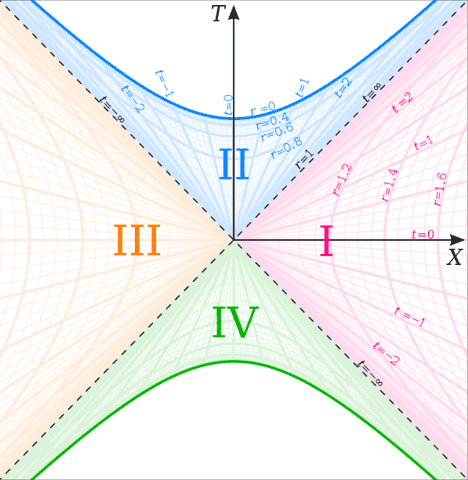
This line element is very interesting. Notice, first, that it is diagonal, just like in Schwarzschild coordinates, but unlike those coordinates, the coefficients of $dT^2$ and $dX^2$ have the same magnitude (and they are nonzero for all positive $r$). And since the angular part of the line element is just the standard metric on a 2-sphere, as before, we have an easy interpretation of what these coordinates are telling us: a small patch of spacetime in these coordinates looks just like a small patch of Minkowski spacetime, and the only difference between two small patches centered on different points is the scaling of the $T$ and $X$ coordinates. In particular, radial light rays are 45 degree lines in these coordinates, just as they are in Minkowski coordinates, so it is easy to see the causal structure. In short, we can draw a spacetime diagram of Schwarzschild spacetime in these coordinates that looks like the spacetime diagrams we are used to in SR. The diagram looks like this:

What’s more, drawing such a diagram can help us to visualize the distortion in Schwarzschild coordinates near $r = 2M$ that we talked about in the last article. First, we need the following useful expressions that relate the Schwarzschild $r$ and $t$ to $T$ and $X$:

$$
T^2 – X^2 = \left( 1 – \frac{r}{2M} \right) e^{r/2M}
$$

$$
\frac{T}{X} = \tanh \left( \frac{t}{4M} \right) \text{ ( for } r > 2M \text{ )}
$$

$$
\frac{X}{T} = \tanh \left( \frac{t}{4M} \right) \text{ ( for } r < 2M \text{ )}
$$

With these expressions, we can see that curves of constant $r$ are hyperbolas in our spacetime diagram, except for $r = 2M$, which is the pair of 45 degree lines that meet at the origin. And curves of constant $t$ are just straight lines through the origin, whose slope up and to the right increases from horizontal for $t = 0$ to 45 degrees for $t \rightarrow \infty$; then, for slopes greater than 45 degrees, $t$ is decreasing again until the vertical line through the origin is again $t = 0$. If we keep going further, to lines sloped up and to the left, $t$ continues to decrease, and the other 45 degree line corresponds to $t \rightarrow – \infty$; then $t$ increases again until we are back to the horizontal line through the origin, $t = 0$.

There are plenty of implications of all this, many of which we will save for the next article; but one key thing that jumps out at us is that the pair of 45 degree lines through the origin are lines of constant $r$ and constant $t$! (Well, “constant” $t$ of $\infty$ or $- \infty$, which technically means $t$ is undefined, but that doesn’t affect the point we are about to make.) So if we think of “grid squares” in Schwarzschild coordinates, which will indeed be squares on our spacetime diagram for very large $r$, as $r$ gets closer to $2M$, the “squares” become squashed into rhombuses that get narrower and narrower, until at $r = 2M$, they have collapsed completely. In short, we simply don’t have a valid Schwarzschild coordinate grid at $r = 2M$, and close to that point the grid is so squashed as to be practically useless. That is the distortion we talked about in the last article, and the Kruskal-Szekeres spacetime diagram lets us actually visualize it, as promised.

In the next article, we’ll look at what else our spacetime diagram in Kruskal-Szekeres coordinates tells us, particularly about the region $r < 2M$.

References

(1) The Wikipedia article on Kruskal-Szekeres coordinates, from which the spacetime diagram is taken:

Wikipedia article on Kruskal-Szekeres coordinates

The image was authored by Dr Greg, Wikimedia Commons (yes, the PF Science Advisor DrGreg).

(2) The Creative Commons License:

Creative Commons License