Weak Values Part 1: Asking Photons Where They Have Been

In a previous Insight on retrocausality, I explained an experiment by Danan, Farfurnik, Bar-Ad, and Vaidman (DFBV)[1], “Asking Photons Where They Have Been” using various retrocausal models. In this Insight, I will give a brief introduction to the formalism for computing the relative power spectra in that experiment. Specifically, I will show how the weak values[2] give the first-order approximation to the probability amplitudes per the full wave function and that one may also compute these amplitudes using the corresponding approximate path integral formalism. As I pointed out in the Insight on retrocausality (references therein), the three analyses that follow correspond to the Transactional Interpretation (TI) or Possibilist Transactional Interpretation (PTI), the Two-State Vector Formulation, and Relational Blockworld or Wharton’s Lagrangian-Only approach, respectively.

Per the DFBV Appendix and Saldanha[3], the full wave function without mirror oscillations for their Figure 1A (below) is

\begin{equation} \Psi (x,y,z,t) \propto e^{-\frac{\left( x^2 + y^2 \right)}{2 \Delta^2 }} \mbox{cos} \left(kz – \omega t \right) \label{fullpsi} \end{equation}

where x and y are transverse to the beam along z. For this experiment $\omega = 2 \pi c/ \lambda$ with $\lambda = 785nm$. The focus of the experiment is on the relative power spectra of weak transverse amplitude vibrations of the mirrors imprinted on the strong longitudinal signal at detector D. DFBV use this information to “ask the photons where they were” in the interferometer between the Source and detector D in various experimental configurations. The presence of small peaks in the signal at D associated with various transverse mirror oscillations is then used to infer an answer to their question via weak values of the Two-State Vector Formulation (TSVF) of quantum mechanics. Therefore, we need only study the transverse component of the wave function in the direction of mirror oscillation (y).

The wave function for displacement transverse to the beam line along which the mirrors vibrate (y) for their Figure 1A is

\begin{equation} \Psi (y) \propto \left( e^{-\frac{\left( y – \delta_C \right)^2 }{2 \Delta^2 }} + e^{-\frac{\left( y – \delta_E – \delta_A – \delta_F \right)^2 }{2 \Delta^2 }} + e^{-\frac{\left( y – \delta_E – \delta_B – \delta_F \right)^2 }{2 \Delta^2 }} \right) \label{Fig1A} \end{equation}

where $\delta_X = \delta \mbox{sin} \left( 2 \pi f_X t \right)$ is the oscillatory function for each mirror with $\delta = (0.6\mu m)$ (displacement of beam at detector due to mirror oscillations) and $\Delta = 1.2 mm$ (size of beam at the detector) with mirror oscillatory frequencies of 282 Hz, 296 Hz, 307 Hz, 318 Hz, and 332 Hz, for mirrors A, B, C, E, and F, respectively. That $\delta \ll \Delta$ means we have a so-called “weak measurement.” The wave function for their Figure 1B (below) is

\begin{equation} \Psi (y) \propto \left( e^{-\frac{\left( y – \delta_C \right)^2 }{2 \Delta^2 }} + e^{-\frac{\left( y – \delta_E – \delta_A – \delta_F \right)^2 }{2 \Delta^2 }} – \: e^{-\frac{\left( y – \delta_E – \delta_B – \delta_F \right)^2 }{2 \Delta^2 }} \right) \label{Fig1B} \end{equation}

And the wave function for their Figure 1C (below) is

\begin{equation} \Psi (y) \propto \left( e^{-\frac{\left( y – \delta_E – \delta_A – \delta_F \right)^2 }{2 \Delta^2 }} – \: e^{-\frac{\left( y – \delta_E – \delta_B – \delta_F \right)^2 }{2 \Delta^2 }} \right) \label{Fig1C} \end{equation}

The signal strength S is analyzed by differencing the integrated signal about the center of the detector face 2,500 times a second, i.e.,

\begin{equation} S = \int_{y > 0} \mid \Psi (y) \mid ^2 dy \: – \int_{y < 0} \mid \Psi (y) \mid ^2 dy \label{S} \end{equation}

Expanding Eq(\ref{Fig1A}) to first order in $\delta_X$ we have

\begin{equation} \Psi (y) \approx e^{- \frac{y^2}{2 \Delta ^2}}  \left( 3 + \frac{y}{\Delta ^2} \left( \delta_C + \delta_A + \delta_B + 2 \delta_E + 2 \delta_F  \right) \right) \label{Psi1A} \end{equation}

which means

\begin{equation} \mid \Psi (y) \mid ^2 \approx e^{- \frac{y^2}{ \Delta ^2}}  \left( 9 + \frac{6y}{\Delta ^2} \left( \delta_C + \delta_A + \delta_B + 2 \delta_E + 2 \delta_F  \right) \right) \label{Psi1Ab} \end{equation}

and

\begin{equation} S \sim \delta_C + \delta_A + \delta_B + 2 \delta_E + 2 \delta_F  \label{S1A} \end{equation}

I used MATLAB to do a fast Fourier transform of S at x = 0 per equation 21 in DFBV’s Supplement IV for $\Psi$ of their equation 23, i.e., Eq(\ref{Fig1A}) times $\frac{1}{3\sqrt{3}}$ in Eq(\ref{S}) (Figure 3). This shows the 2:1 ratio of amplitudes for mirror frequencies per Eq(\ref{S1A}). When you square S in Eq(\ref{S1A}) using $\delta_X = \mbox{sin} \left( 2 \pi f_X t \right)$ and integrate from 0 to 1 second, the cross terms  are zero. Thus, the power spectrum goes as the square of the individual amplitudes (their Figure 1A below).

Expanding Eq(\ref{Fig1B}) to first order in $\delta_X$ we have
\begin{equation} \Psi (y) \approx e^{- \frac{y^2}{2 \Delta ^2}}  \left( 1 + \frac{y}{\Delta ^2} \left( \delta_C + \delta_A – \delta_B \right) \right) \label{Psi1B} \end{equation}

which means

\begin{equation} \mid \Psi (y) \mid ^2 \approx e^{- \frac{y^2}{ \Delta ^2}}  \left( 1 + \frac{2y}{\Delta ^2} \left( \delta_C + \delta_A – \delta_B  \right) \right) \label{Psi1Bb} \end{equation}

and

\begin{equation} S \sim \delta_C + \delta_A – \delta_B   \label{S1B} \end{equation}

I used MATLAB to do a fast Fourier transform of S at x = 0 per equation 21 in DFBV’s Supplement IV for $\Psi$ of their equation 20, i.e., Eq(\ref{Fig1B}) times $\frac{1}{3}$ in Eq(\ref{S}) (Figure 4). This shows the 1:1 ratio of amplitudes for mirror frequencies A, B, and C with zero amplitudes for mirror frequencies E and F per Eq(\ref{S1B}). Again, the power spectrum then goes as the relative squares of the amplitudes as in their Figure 1B below.

Expanding Eq(\ref{Fig1C}) to first order in $\delta_X$ we have \begin{equation} \Psi (y) \approx e^{- \frac{y^2}{2 \Delta ^2}}  \left( \frac{y}{\Delta ^2} \left( \delta_A – \delta_B \right) \right) \label{Psi1C} \end{equation}

which means

\begin{equation} \mid \Psi (y) \mid ^2 \approx 0 \label{Psi1Cb} \end{equation}

i.e., there are no first-order terms, so there is no first-order contribution to S.

Notice that while there is photon leakage from mirror F in the configuration of Figure 1C, there is no main beam on which that signal can supervene due to the destructive interference between mirrors A and B and mirror F. This destructive interference in the main beam is represented mathematically by the cancellation of the 1’s in obtaining Eq(\ref{Psi1C})

\begin{equation} e^{\frac{y \delta_A }{\Delta ^2}} – e^{\frac{y \delta_B }{\Delta ^2}} \approx 1 + \frac{y \delta_A }{\Delta ^2} – 1 – \frac{y \delta_B }{\Delta ^2} = \frac{y \delta_A }{\Delta ^2} –\frac{y \delta_B }{\Delta ^2}  \label{Psi1Cc} \end{equation}

Without a constant term the square of this $\Psi(y)$ doesn’t result in any linear terms in $\delta_X$ which means there are no linear terms in the corresponding signal S and the leaking photons do not produce peaks above the noise (Figure 1C). That the lowest-order contribution to the signal from mirrors A and B in this case is second order instead of first order means they do not contribute to the weak measurement as seen in the corresponding weak values. In fact, this linearity is a hallmark of weak values. When it is possible to obtain weak values with second-order contributions their ontological implications become suspect, as we will see in the next Insight (Weak Values Part 2) on the quantum Cheshire Cat experiment of Denkmayr et al.

I used MATLAB to do a fast Fourier transform of S at x = 0 per equation 21 in DFBV’s Supplement IV for $\Psi$ of their equation 22, i.e., Eq(\ref{Fig1C}) times $\frac{1}{3}$ in Eq(\ref{S}) (Figure 5). Figure 5 is scaled to Figures 3 and 4, so no amplitudes are seen. If you allow for small enough scaling, several peaks can be seen (Figure 6), including frequencies for mirrors A, B, E, and F, but nothing for mirror C.

Now let’s look at the corresponding weak values for these three weak measurements.

The weak value for operator O is defined as

\begin{equation} \langle O \rangle _W \equiv \frac{\langle \Phi \mid O \mid \Psi \rangle}{\langle \Phi \mid \Psi \rangle} \label{WV} \end{equation}

$\langle \Phi \mid$ is called the “post-selected state” and evolves from the detection event at D backward in time to the emission event at the Source. [TI and PTI also employ a retrocausal wave in constructing $\mid \Psi \mid ^2$ as described in my Insight on retrocausality.] $\mid \Psi \rangle$ is called the “pre-selected state” and evolves forward in time from the emission event at the Source to the detection event at D. We want the weak values for projection operators at each mirror X, i.e., $\mid X \rangle \langle X \mid$. For mirrors A, B, and C in Figure 1A we have

\begin{equation} \langle \Phi \mid = \frac{1}{\sqrt{3}} \left( \langle A \mid + \langle B \mid + \langle C  \mid \right) \label{Fig1Astate1} \end{equation}

and

\begin{equation} \mid \Psi \rangle = \frac{1}{\sqrt{3}} \left( \mid A \rangle + \mid B \rangle + \mid C  \rangle \right) \label{Fig1Astate2} \end{equation}

Using $\langle X \mid X \rangle = 1$ and $\langle X \mid Y \rangle = 0$ we have $\langle \Phi \mid \Psi \rangle = 1$. Thus, the weak value for the projection operator at mirror A in Figure 1A is

\begin{equation} \langle P_A \rangle _W = \frac{1}{\sqrt{3}} \left( \langle A \mid + \langle B \mid + \langle C  \mid \right) \mid A \rangle \langle A \mid \frac{1}{\sqrt{3}} \left( \mid A \rangle + \mid B \rangle + \mid C  \rangle \right) = \frac{1}{3} \label{Aweak} \end{equation}

Obviously, we get the same result for mirrors B and C. For mirror E in Figure 1A we have

\begin{equation} \langle \Phi \mid = \frac{1}{\sqrt{3}} \left( \sqrt{2} \langle E \mid + \langle C  \mid \right) \label{Fig1Astate3} \end{equation}

and

\begin{equation} \mid \Psi \rangle = \frac{1}{\sqrt{3}} \left( \sqrt{2} \mid E \rangle + \mid C  \rangle \right) \label{Fig1Astate4} \end{equation}

Replacing E with F gives $\langle \Phi \mid$ and $\mid \Psi \rangle$ for mirror F. Again, we have $\langle \Phi \mid \Psi \rangle = 1$, so the weak value for the projection operator at mirror E in Figure 1A is

\begin{equation} \langle P_E \rangle _W = \frac{1}{\sqrt{3}} \left( \sqrt{2} \langle E \mid + \langle C  \mid \right)\mid E \rangle \langle E \mid \frac{1}{\sqrt{3}} \left( \sqrt{2} \mid E \rangle + \mid C  \rangle \right) = \frac{2}{3} \label{Eweak} \end{equation}

Obviously, we get the same result for mirror F. [The factors of $\frac{\sqrt{2}}{\sqrt{3}}$ and $\frac{1}{\sqrt{3}}$ are there because the first beam splitter sends $\frac{1}{3}$ of the signal to mirror C and $\frac{2}{3}$ to mirror E (it’s a 1-2 beam splitter). The last beam splitter recombines the signal in the same manner. The other two beam splitters in the inner interferometer are 1-1, i.e., divide the signal in half. Thus, the same signal strength appears at mirrors A, B, and C.] Notice that the relative sizes of these weak values match exactly the relative amplitudes of the $\delta_X$ in S of Eq(\ref{S1A}). This is not mere coincidence, but obtains by design. The experiment was designed so that the transverse mirror oscillation frequencies could supervene on and not interrupt the longitudinal signal of much greater strength thereby acting as tags on the longitudinal signal to answer the question, “Where have the photons been between emission at the Source and detection at D?” Therefore, the relative intensity (as seen in the power spectra) of the transverse mode for each mirror is equal to the relative intensity of the longitudinal mode associated with each mirror as reproduced by the weak values. This relative intensity can also be produced for the longitudinal mode of each mirror using the path integral per Sinha & Sorkin[4] or Wharton et al.[5], for example. I will do that after finishing the weak values for the various configurations of Figures 1A-C. Next I’ll compute the weak values for Figure 1B.

For mirrors A, B, and C in Figure 1B we have

\begin{equation} \langle \Phi \mid = \frac{1}{\sqrt{3}} \left( \langle A \mid + i \langle B \mid + \langle C  \mid \right) \label{Fig1Bstate1} \end{equation}

and

\begin{equation} \mid \Psi \rangle = \frac{1}{\sqrt{3}} \left( \mid A \rangle + i \mid B \rangle + \mid C  \rangle \right) \label{Fig1Bstate2} \end{equation}

Notice these only differ from Eqs(\ref{Fig1Astate1} & \ref{Fig1Astate2}) by the factor $i$ to account for the changed phase between mirror B and the second beam splitter in the inner interferometer creating destructive interference between mirrors A and B and mirror F. We now have $\langle \Phi \mid \Psi \rangle = \frac{1}{3}$, so $\langle P_A \rangle _W = \langle P_C \rangle _W = 1$ and $\langle P_B \rangle _W = -1$.  For mirror E in Figure 1B we have

\begin{equation} \langle \Phi \mid = \frac{1}{\sqrt{3}} \langle C  \mid \label{Fig1Bstate3} \end{equation}

and

\begin{equation} \mid \Psi \rangle = \frac{1}{\sqrt{3}} \left( \sqrt{2} \mid E \rangle + \mid C  \rangle \right) \label{Fig1Bstate4} \end{equation}

The difference between these states and those of Eqs(\ref{Fig1Astate3} & \ref{Fig1Astate4}) is seen in their Figure 1E (below). The backward evolving wave $\langle \Phi \mid$ no longer reaches mirror E as represented by Eq(\ref{Fig1Bstate3}). Thus, $\langle P_E \rangle _W = 0$. A similar situation obtains for mirror F where

\begin{equation} \langle \Phi \mid = \frac{1}{\sqrt{3}}  \left( \sqrt{2} \langle F \mid + \langle C  \mid \right) \label{Fig1Bstate5} \end{equation}

and

\begin{equation} \mid \Psi \rangle = \frac{1}{\sqrt{3}} \mid C  \rangle \label{Fig1Bstate6} \end{equation}

Again, looking at Figure 1E you see that the forward evolving wave $\mid\Psi \rangle$ does not reach mirror F as represented by Eq(\ref{Fig1Bstate6}). Thus, $\langle P_F \rangle _W = 0$. Again, the relative sizes of these weak values match exactly the relative sizes of the $\delta_X$ in S of Eq(\ref{S1B}).

For mirrors A, B, and C in Figure 1C we have

\begin{equation} \langle \Phi \mid = \frac{1}{\sqrt{3}} \left( \langle A \mid + i \langle B \mid + \langle Absorbed  \mid \right) \label{Fig1Cstate1} \end{equation}

and

\begin{equation} \mid \Psi \rangle = \frac{1}{\sqrt{3}} \left( \mid A \rangle + i \mid B \rangle + \mid C  \rangle \right) \label{Fig1Cstate2} \end{equation}

Notice that now the weak values are undefined because $\langle \Phi \mid \Psi \rangle = 0$ in the denominator of Eq(\ref{WV}), the definition of weak values. This is simply telling us that there is no signal upon which the weak values can supervene[6]. So, even though their Figure 2C (below) shows the presence of photons at mirrors A and B, there is no signal at detector D (no double line, no photons) so the weak values for mirrors A, B, and C are zero[7]. For mirror E, the forward evolving wave would contain contributions from mirrors E and C (same as Eq(\ref{Fig1Bstate4})), but the backward evolving wave would be zero, since the backward evolving wave is absorbed before reaching mirror C changing Eq(\ref{Fig1Bstate3}) to read $\langle \Phi \mid = 0$. For mirror F, the forward evolving wave would be the same as Eq(\ref{Fig1Bstate6}) while the backward evolving wave would contain only a contribution from mirror F, i.e., $\langle \Phi \mid = \frac{1}{\sqrt{3}}  \left( \sqrt{2} \langle F \mid + \langle Absorbed  \mid \right)$. Thus, as with the weak values for mirrors A, B, and C, we have $\langle \Phi \mid \Psi \rangle = 0$ for mirrors E and F in the configuration of Figure 1C. In this case, there are no photons at all reaching mirrors E and F (like the case for mirror C) per their Figure 2C, so one wouldn’t expect to see any evidence thereof even if you had a signal at detector D upon which to supervene. Finally, let’s see what the path integral formalism has to say.

The path integral formalism produces an amplitude $\Psi_f(z)$ using the classical action $S(z’,z)$ (where again z is the longitudinal coordinate) as follows[8]

\begin{equation} \Psi_f(z) = \int e^{iS(z’,z)/ \hbar} \Psi_i(z’) dz’ \label{PI} \end{equation}

We assume a point Source at z‘ = 0 so $\Psi_i(z’) = \delta (z’)$ and $\Psi_f(z) = e^{iS(0,z)/ \hbar}$. The classical action for the wave is just $S(z’,z) = 2 \pi \frac{z – z’}{\lambda}\hbar$ where $\lambda$ is the wavelength (the DeBroglie wavelength in the case of matter waves as in Bach et al.[8]). That is, $\frac{S(z’,z)}{\hbar}$ is just the phase of the wave at z relative to z’ and in this case we’re using z’ = 0. We’re only concerned with phase differences between various paths, so our amplitudes will only need to account for those, e.g., Sinha & Sorkin[4] and Wharton et al.[5]. Thus, we need only account for the fact that reflection introduces a phase difference of $\pi /2$ leading to a factor of $i = e^{i \pi /2}$ in the amplitude, the first and last 1-2 beam splitters introduce factors of $\frac{\sqrt{2}}{\sqrt{3}}$ and $\frac{1}{\sqrt{3}}$ (as explained above), the 1-1 beam splitters introduce a factor of $\frac{1}{\sqrt{2}}$, and changing the path length from the configuration of Figure 1B to that of 1A means an additional factor of $-1 = e^{i \pi}$ in the amplitude from mirror B in order to get constructive interference with the signal from mirror A to mirror F. Accordingly, the amplitude associated with mirror A in Figure 1A is[9]

\begin{equation} \left(i \frac{\sqrt{2}}{\sqrt{3}} \right) \left(i\right)\left(i \frac{1}{\sqrt{2}}\right)\left( i\frac{1}{\sqrt{2}}\right) \left(i\right) \left(i \frac{\sqrt{2}}{\sqrt{3}} \right) = \: – \frac{1}{3} \label{Fig1AA} \end{equation}

Reading from left to right in each pair of parentheses connecting the Source to mirror A we have contributions from (reflection at the first 1-2 beam splitter)(reflection from mirror E)(reflection from a 1-1 beam splitter). Continuing left to right to connect mirror A to detector D we have contributions from (reflection at a 1-1 beam splitter)(reflection at mirror F)(reflection at the last 1-2 beam splitter). There is no difference between this amplitude for A and the amplitude for A in Figure 1B. We have for mirror B in Figure 1A

\begin{equation} \left(i \frac{\sqrt{2}}{\sqrt{3}} \right) \left(i\right)\left(\frac{1}{\sqrt{2}}\right)\left(-1\right)\left(\frac{1}{\sqrt{2}}\right) \left(i\right) \left(i \frac{\sqrt{2}}{\sqrt{3}} \right) = \: – \frac{1}{3} \label{Fig1AB} \end{equation}

Reading from left to right in each pair of parentheses connecting the Source to mirror B we have contributions from (reflection at the first 1-2 beam splitter)(reflection from mirror E)(transmission at a 1-1 beam splitter). Continuing left to right to connect mirror B to detector D we have contributions from (phase to get constructive interference to mirror F)(transmission at a 1-1 beam splitter)(reflection at mirror F)(reflection at the last 1-2 beam splitter). The only difference between the configuration of Figure 1A and that of Figure 1B is the factor (phase to get constructive interference to mirror F), so that the amplitude for mirror B in Figure 1B is $\frac{1}{3}$. We have for mirror C in Figure 1A

\begin{equation} \left(\frac{1}{\sqrt{3}} \right)\left(-1\right) \left(\frac{1}{\sqrt{3}} \right)  = \: -\frac{1}{3} \label{Fig1AC} \end{equation}

Reading from left to right in each pair of parentheses connecting the Source to mirror C we have only a contribution from (transmission at a 1-2 beam splitter). Continuing left to right to connect mirror C to detector D we have (phase to get constructive interference to detector D)(transmission at a 1-2 beam splitter). This is also the amplitude for mirror C in the configuration of Figure 1B. We have for mirror E in Figure 1A

\begin{equation} \left(i \frac{\sqrt{2}}{\sqrt{3}} \right) \left(\left(i \frac{1}{\sqrt{2}}\right)\left(i\right)\left( i\frac{1}{\sqrt{2}}\right) \left(i\right) \left(i \frac{\sqrt{2}}{\sqrt{3}} \right) +\left(\frac{1}{\sqrt{2}}\right) \left(i\right)\left(-1\right)\left(\frac{1}{\sqrt{2}}\right) \left(i\right) \left(i \frac{\sqrt{2}}{\sqrt{3}} \right)\right) = \: – \frac{2}{3} \label{Fig1AE} \end{equation}

Reading from left to right in each pair of parentheses connecting the Source to mirror E we have only a contribution from (reflection at the first 1-2 beam splitter). Then there are two paths needed to connect mirror E with detector D, i.e., (reflection at a 1-1 beam splitter)(reflection at mirror A)(reflection at a 1-1 beam splitter)(reflection at mirror F)(reflection at a 1-2 beam splitter) plus (transmission at a 1-1 beam splitter)(reflection at mirror B)(phase to get constructive interference to mirror F)(transmission at a 1-1 beam splitter)(reflection at mirror F)(reflection at the last 1-2 beam splitter). The only difference between the configuration of Figure 1A and that of Figure 1B is the factor (phase to get constructive interference to mirror F), so that the amplitude for mirror E in Figure 1B is

\begin{equation} \left(i \frac{\sqrt{2}}{\sqrt{3}} \right) \left(\left(i \frac{1}{\sqrt{2}}\right)\left(i\right)\left( i\frac{1}{\sqrt{2}}\right) \left(i\right) \left(i \frac{\sqrt{2}}{\sqrt{3}} \right) +\left(\frac{1}{\sqrt{2}}\right) \left(i\right)\left(\frac{1}{\sqrt{2}}\right) \left(i\right) \left(i \frac{\sqrt{2}}{\sqrt{3}} \right)\right) = \: 0 \label{Fig1BE} \end{equation}

The same results obtain for mirror F where in Figure 1A we have

\begin{equation} \left(\left(i \frac{\sqrt{2}}{\sqrt{3}} \right)\left(i\right)\left(i \frac{1}{\sqrt{2}}\right)\left(i\right)\left( i\frac{1}{\sqrt{2}}\right) + \left(i \frac{\sqrt{2}}{\sqrt{3}} \right)\left( i\right)\left(\frac{1}{\sqrt{2}}\right) \left(i\right)\left(-1\right)\left(\frac{1}{\sqrt{2}}\right)\right) \left(i \frac{\sqrt{2}}{\sqrt{3}} \right) = \: – \frac{2}{3} \label{Fig1AF} \end{equation}

Reading from left to right in each pair of parentheses connecting the Source to mirror F we have contributions from two paths, i.e., (reflection at the first 1-2 beam splitter)(reflection at mirror E)(reflection at a 1-1 beam splitter)(reflection at mirror A)(reflection at a 1-1 beam splitter) plus (reflection at the first 1-2 beam splitter)(reflection at mirror E)(transmission at a 1-1 beam splitter)(reflection at mirror B)(phase to get constructive interference to mirror F)(transmission at a 1-1 beam splitter). Then to connect mirror F with detector D we have (reflection at the last 1-2 beam splitter). The only difference between the configuration of Figure 1A and that of Figure 1B is the factor (phase to get constructive interference to mirror F), so that the amplitude for mirror F in Figure 1B is

\begin{equation} \left(\left(i \frac{\sqrt{2}}{\sqrt{3}} \right)\left(i\right)\left(i \frac{1}{\sqrt{2}}\right)\left(i\right)\left( i\frac{1}{\sqrt{2}}\right) + \left(i \frac{\sqrt{2}}{\sqrt{3}} \right)\left( i\right)\left(\frac{1}{\sqrt{2}}\right) \left(i\right)\left(\frac{1}{\sqrt{2}}\right)\right) \left(i \frac{\sqrt{2}}{\sqrt{3}} \right) = \: 0 \label{Fig1BF} \end{equation}

The path integral computation of amplitudes gives the same results for relative intensity as Eqs(\ref{S1A} & \ref{S1B}). These computations also show us why the factors of $\frac{1}{9}$ and $\frac{4}{9}$ appear in the relative intensities. If you use the rules for path integral amplitudes above and compute, say, the amplitude for Figure 1A from the Source to detector D through both the outer and inner interferometers you get an amplitude of $-i\frac{2}{3} + -i\frac{1}{3} = -i$ from that last 1-2 beam splitter towards detector D and an amplitude of $\frac{\sqrt{2}}{3} + -\frac{\sqrt{2}}{3} = 0$ proceeding down from the last 1-2 beam splitter. Now suppose you adjust the path length from mirror C to the last 1-2 beam splitter so as to obtain constructive interference down (instead of to the right) from the last beam splitter, as was done between mirrors B and F in Figure 1B. In that case the amplitude from the last 1-2 beam splitter towards detector D would be $-i\frac{2}{3} + i\frac{1}{3} = -i\frac{1}{3}$ and the amplitude proceeding down from the last 1-2 beam splitter would be $\frac{\sqrt{2}}{3} + \frac{\sqrt{2}}{3} = \frac{2\sqrt{2}}{3}$. These give relative intensities of $\frac{1}{9}$ and $\frac{8}{9}$, respectively. If you then adjust the path length between mirrors B and F so that you have destructive interference to mirror F (as in Figure 1B), then regardless of the path length between mirror C and the last 1-2 beam splitter the amplitude from the last 1-2 beam splitter to detector D is $\pm i\frac{1}{3}$ and the amplitude proceeding down from the last 1-2 beam splitter is $\pm\frac{\sqrt{2}}{3}$ so that the intensities are $\frac{1}{9}$ and $\frac{2}{9}$, respectively, giving $\frac{1}{3}$ the total signal[10]. Likewise, if you block the signal from mirror C and have constructive interference to mirror F, then the amplitude from the last 1-2 beam splitter to detector D is $- i\frac{2}{3}$ and the amplitude proceeding down from the last 1-2 beam splitter is $-\frac{\sqrt{2}}{3}$ so that the intensities are $\frac{4}{9}$ and $\frac{2}{9}$, respectively, giving $\frac{2}{3}$ the total signal. Thus, we see that the values of S given by Eqs(\ref{S1A} & \ref{S1B}) are indeed the relative amplitudes in the time domain even though we already squared $\Psi(y)$ and integrated in the space domain to get S.

Finally, for the configuration of Figure 1C it is easy to see that we have zero amplitude for mirror C and that Eqs(\ref{Fig1AA}, \ref{Fig1AB}, \ref{Fig1BE}, & \ref{Fig1BF}) still give the amplitudes for mirrors A, B, E, and F (with caveat noted for mirror B), respectively. Thus, as with the other two approaches, we have to note that even though there are non-zero amplitudes for mirrors A and B, there is no strong longitudinal signal upon which these weak transverse signals can imprint, so these signals do not rise above the noise.

In part 2 of the Insights on weak values, I will use the so-called quantum Cheshire Cat experiment of Denkmayr et al. to show that weak values can be obtained with second-order interaction if that interaction contributes equally with first-order interaction to the intensity. However, in that case, the contribution from the second-order interaction destroys the implications of the weak values.

 

 

 

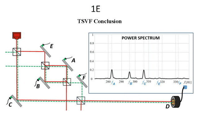
Figure 2C

 

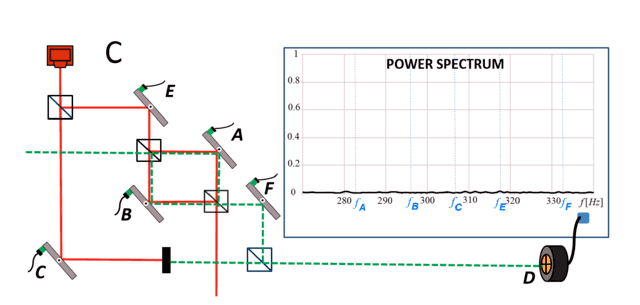
Figure 3

 

Figure 4

Figure 5

Figure 6

 

1. Danan, A., Farfurnik, D., Bar-Ad, S., & Vaidman, L.: Asking Photons Where They Have Been. Physical Review Letters 111, 240402 (2013) http://arxiv.org/abs/1304.7469.
2. Aharonov, Y., Albert, D., & Vaidman, L.: How the result of a measurement of a component of the spin of a spin-1/2 particle can turn out to be 100. Physical Review Letters 60, 1351-1354 (1988); Duck, I., Stevenson, P., & Sudarshan, E.: The sense in which a ‘weak measurement’ of a spin-1/2 particle’s spin component yields a value 100. Physical Review D 40, 2112–2117 (1989); Ritchie, N., Story, J., & Hulet, R.: Realization of a measurement of a ‘weak value’. Physical Review Letters 66, 1107–1110 (1991); Dressel, J., Malik, M., Miatto, F., Jordan, A., & Boyd, R.: Colloquium: understanding quantum weak values: basics and applications. Reviews of Modern Physics 86, 307–316 (2014).
3. Saldanha, P.: Interpreting a nested Mach-Zehnder interferometer with classical optics. Physical Review A 89, 033825 (2014) http://arxiv.org/abs/1312.7438.
4. Sinha, S., & Sorkin, R.: A Sum-Over-Histories Account of an EPR(B) Experiment. Foundations of Physics Letters 4, 303-335 (1991).
5. Wharton, K., Miller, D., & Price, H.: Action Duality: A Constructive Principle for Quantum Foundations. Symmetry 3, 524-540 (2011).
6. See the Opinion, “Asking photons where they have been without telling them what to say,” by Hatim Salih in Frontiers of Physics: Optics and Photonics, 5 December 2014, and “Reply to a Commentary ‘Asking photons where they have been without telling them what to say,’” by Ariel Danan, Demitry Farfurnik, Shimshon Bar-Ad, and Lev Vaidman in Frontiers of Physics: Optics and Photonics, 22 April 2015.
7. DFBV point out there are leakage photons reaching detector D from mirrors A and B, but that signal is too small to be seen above the noise.
8. Bach, R., Pope, D., Sy-Hwang, L., & Batelaan, H.: Controlled double-slit electron diffraction. New Journal of Physics 15, 033018 (2013). See section 3 of the Supplementary Information.
9. Stuckey, W.M., Silberstein, M., & McDevitt, T.: Relational Blockworld: Providing a Realist Psi-Epistemic Account of Quantum Mechanics. International Journal of Quantum Foundations 1, No. 3, 123-170 (2015) http://www.ijqf.org/wps/wp-content/uploads/2015/06/IJQF2015v1n3p2.pdf.
10. This is why DFBV point out that the signal for Figure 1A would be 9 times stronger than the signal for Figure 1B unless they adjusted the Source.