Analyzing Hysteresis Curve Fitting: Overfitting or Not?

[Wrichik Basu]

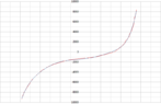
We recently did an experiment to generate the hysteresis curve of a certain material. The experiment involved switching the current in the wire looped around a ring of the material, and recording the first throw of the ballistic galvanometer. I am not going into the details of calculations because the thread is intended to be regarding curve fitting. After certain calculations, we arrived at the following data for a graph of B vs H (in MATLAB):

B = [1.389 1.374 1.345 1.331 1.316 1.302 1.287 1.273 1.258 1.229 1.215 1.215 1.172 1.128 1.114 ...
     1.099 1.056 1.041 1.027 1.013 0.984 0.969 0.969 0.955 0.839 0.448 0.391 0.275 0.130 -0.275 ...
    -0.405 -0.579 -0.665 -0.781 -0.839 -0.882 -0.955 -0.998 -1.114 -1.201 -1.244 -1.287 -1.345 ...
    -1.403 -1.432 -1.461];

H = [8409.911 7488.684 6805.193 6181.136 5289.626 5022.173 4695.286 4249.531 3982.078 3744.342 ...
    3417.455 3090.568 2644.813 2258.492 2020.756 1753.303 1426.416 1248.114 1129.246 980.661 ...
    921.227 832.076 772.642 653.774 0.000 -861.793 -950.944 -1069.812 -1218.397 -1575.001 -1842.454 ...
    -2228.775 -2466.511 -2823.115 -3090.568 -3328.304 -3595.757 -3952.361 -4784.437 -5438.211 ...
    -6002.834 -6567.457 -7250.948 -8053.307 -8558.496 -9331.138];

Note that this is only half of the hysteresis curve; the other half is to be plotted by symmetry.

I am supposed to find the best fit curve for this data. Some further calculations need to be done on the area between the two curves.

For non-linear regression, I generally use the Shape Language Modelling tool available on MATLAB File Exchange. I am creating the model as follows:

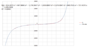
slm = slmengine(H, B, 'increasing', 'on', 'concaveup', 'on', 'knots', no_of_knots);

concaveup is the curvature constraint — the second derivative should never be negative, while increasing is the monotonicity constraint.

I can get different shapes of curves by choosing different values for the number of knots. The default is 6. If I increase the number of knots, the root-mean-square error (RMSE) decreases until it reaches no_of_knots = 70, after which it increases and the curve becomes garbage. In the Imgur post below, I have shown the curves for different number of knots. The RMSE for each curve is also shown on the plot. The dashed blue line is the other half of the hysteresis loop, generated by a centre of inversion symmetry.

​

The curves with higher number of knots seem to be closer to the data points. However, looking at the unevenness of the curve near the bottom, I was wondering if I am overfitting the data? Should I blindly go with the RMSE and choose the curve with 70 knots, or am I indeed overfitting and should choose a knots value somewhere in the middle?

 

[Dale]

To me it looks like your model is not very good. There does not seem to be much benefit in going from 20 to 70 knots, but even 20 degrees of freedom is a lot for the shape. There simply is not a lot of detail in this shape, so it seems like you should be able to find a model that fits better with much fewer than 20 parameters.

 

[Wrichik Basu]

To me it looks like your model is not very good. There does not seem to be much benefit in going from 20 to 70 knots, but even 20 degrees of freedom is a lot for the shape. There simply is not a lot of detail in this shape, so it seems like you should be able to find a model that fits better with much fewer than 20 parameters.

SLM is the best I could find. polyfit overestimates and diverges very often. nlinfit requires a model and can't fit unknown data.

 

[Frabjous]

What does the concaveup flag do?

 

[Dale]

nlinfit requires a model and can't fit unknown data.

Yes, this is where I think you should spend your effort. I think you should develop the model for this data set. It looks like a pretty standard sigmoid curve, but perhaps with a bit of a steep slope in the middle. I would look for a sigmoid function where the slope in the middle is an explicit parameter.

 

[Dale]

If you don’t want to do that and you really just want to use the SLM, then you may want to see if your packages can calculate one of the information criteria, like the Bayesian information criterion. That could tell you if the extra terms are worth including. I think that would reject the ones more than 20.

 

[TonyStewart]

7th order Polynomial seems just fine with a fit of 0.9992 when you swap BH on the XY axis.
rounded off with H on the Y axis

Here I even extrapolated the trend.

But due to what seems to be measurement error with B on the Y axis with amplified Nth order overshoot. I'm not saying the error was with B but this way errors are reduced.
You can recompute the data and see how much error existed with some of the measurements.

As you observed with B on the Y axis

I used scalc.exe from OpenOffice.

 

[Wrichik Basu]

If you don’t want to do that and you really just want to use the SLM, then you may want to see if your packages can calculate one of the information criteria, like the Bayesian information criterion. That could tell you if the extra terms are worth including. I think that would reject the ones more than 20.

It calculates the following for the model:

>> slm.stats

ans =

  struct with fields:

      TotalDoF: 140
        NetDoF: 72
          RMSE: 0.213177002276494
            R2: 0.994795321464372
         R2Adj: 1.00900809746551
    ErrorRange: [-0.208681839581725 0.178549646418819]
     Quartiles: [-0.00910383272107265 0.0309651907320805]
       finalRP: 0.0001
        YShift: 1.13072434407984
        YScale: 0.350934306674064

 

[TonyStewart]

How do you get a polynomial to have zero slope when extrapolated to large inputs? like for a step function?
Above I showed how to reduce the error by inverting the function. Can you think of another function?

 

[JJacquelin]

By inspection one observes that the shape of the whole curve looks like two arcs of hyperbolas : on the first figure the blue curve for small x and the green curve for large x.

Thus the whole model function can be presented as a picewise function. The equation writen on the second figure involves the Heaviside"s function H(X).

This isn't a smooth curve at the point of jonction. To make it smooth one replace the Heaviside function by a smooth approximate function. The smoothness is controled by the parameter lambda. The value of lambda is not critical on a large range which alows to choose a convenient jonction between the two arcs of hyperbolas : Equation and fitted curve are shown on the second figure.