The Amazing Relationship Between Integration And Euler’s Number

We use integration to measure lengths, areas, or volumes. This is a geometrical interpretation, but we want to examine an analytical interpretation that leads us to Integration reverses differentiation. Hence let us start with differentiation.

Weierstraß Definition of Derivatives

$f$ is differentiable at $x$ if there is a linear map $D_{x}f$, such that
\begin{equation*}
\underbrace{D_{x}(f)}_{\text{Derivative}}\cdot \underbrace{v}_{\text{Direction}}=\left(\left. \dfrac{df(t)}{dt}\right|_{t=x}\right)\cdot v=\underbrace{f(x+v)}_{\text{location plus change}}-\underbrace{f(x)}_{\text{location}}-\underbrace{o(v)}_{\text{error}}
\end{equation*}
where the error $o(v)$ increases slower than linear (cp. Landau symbol). The derivative can be the Jacobi-matrix, a gradient, or simply a slope. It is always an array of numbers. If we speak of derivatives as functions, then we mean $f’\, : \,x\longmapsto D_{x}f.$ Integration is the problem to compute $f$ from $f’$ or $f$ from
$$
\dfrac{f(x+v)-f(x)}{|v|}+o(1)
$$
The quotient in this expression is linear in $f$ so
$$
D_x(\alpha f+\beta g)=\alpha D_x(f)+\beta D_x(g)
$$
If we add the Leibniz rule
$$
D_x(f\cdot g)=D_{x}(f)\cdot g(x) + f(x)\cdot D_{x}(g)
$$
and the chain rule
$$
D_x(f\circ g)=D_{g(x)}(f)\circ g \cdot D_x(g)
$$
then we have the main properties of differentiation.

Integration Rules

The solution $f(x)$ given $D_x(f)$ is written
$$
f(x)=\int D_x(f)\,dx=\int f'(x)\,dx
$$
which is also linear
$$
\int \left(\alpha f'(x)+\beta g'(x)\right)\,dx = \alpha \int f'(x)\,dx +\beta \int g'(x)\,dx
$$
and obeys the Leibniz rule which we call integration by parts
$$
f(x)g(x)=\int D_x(f\cdot g)\,dx=\int f'(x)g(x)\,dx + \int f(x)g'(x)\,dx
$$
and the chain rule leads to the substitution rule of integration
\begin{align*}
f(g(x))=\int f'(g(x))dg(x)&=\int \left.\dfrac{df(y)}{dy}\right|_{y=g(x)}\dfrac{dg(x)}{dx}dx=\int f'(g(x))g'(x)dx
\end{align*}

Differentiation is easy, Integration is difficult

In order to differentiate, we need to compute
$$
D_x(f)=\lim_{v\to 0}\left(\dfrac{f(x+v)-f(x)}{|v|}+o(1)\right)=\lim_{v\to 0}\dfrac{f(x+v)-f(x)}{|v|}
$$
which is a precisely defined task. However, if we want to integrate, we are given a function $f$ and will have to find a function $F$ such that
$$
f(x)=\lim_{v\to 0}\dfrac{F(x+v)-F(x)}{|v|}.
$$
The limit as a computation task is not useful since we do not know $F.$ In fact, we have to consider the pool of all possible functions $F,$ compute the limit, and check whether it matches the given function $f.$ And the pool of all possible functions is large, very large. The first integrals are therefore found by the opposite method: differentiate a known function $F,$ compute $f=D_x(F),$ and list
$$
F=\int D_x(F)\,dx=\int f(x)\,dx.
$$
as an integral formula. Sure, there are numerical methods to compute an integral, however, this does not lead to a closed form with known functions. A big and important class of functions is polynomials. So we start with $F(x)=x^n.$
\begin{align*}
D_x(x^n)&=\lim_{v\to 0}\dfrac{(x+v)^n-x^n}{|v|}=\lim_{v\to 0}\dfrac{\binom n 1 x^{n-1}v+\binom n 2 x^{n-2}v^2+\ldots}{|v|}=nx^{n-1}
\end{align*}
and get
$$
x^n = \int nx^{n-1}\,dx \quad\text{or} \quad \int x^r\,dx = \dfrac{1}{r+1}x^{r+1}
$$
and in particular $\int 0\,dx = c\, , \,\int 1\,dx = x.$ The formula is even valid for any real number $r\neq -1.$ But what is
$$
\int \dfrac{1}{x}\,dx\text{ ?}
$$

Euler’s Number and the $\mathbf{e}-$Function

The history of Euler’s number $\mathbf{e}$ is the history of the reduction of multiplication (difficult) to addition (easy). It runs like a red thread through the history of mathematics, from John Napier (1550-1617) and Jost Bürgi (1552-1632) to Volker Strassen (1936-), Shmuel Winograd (1936-2019) and Don Coppersmith ($\sim$1950 -). Napier and Bürgi published logarithm tables to a base close to $\mathbf{1/e}$ (1614), resp. close to $\mathbf{e}$ (1620) to use
$$
\log_b (x\cdot y)=\log_b x+\log_b y.
$$
Strassen, Coppersmith, and Winograd published algorithms for matrix multiplication that save elementary multiplications at the expense of more additions. Napier and Bürgi were probably led by intuition. Jakob Bernoulli (1655-1705) already found $\mathbf{e}$ in 1669 by the investigation of interest rates calculations. Grégoire de Saint-Vincent (1584-1667) solved the problem about the hyperbola, Apollonius of Perga ($\sim$240$\sim$190 BC).

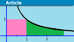
What is the number at the right such that the red and green areas are equal?

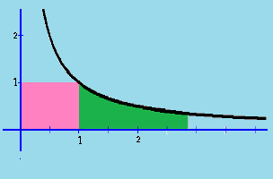
This is in modern terms the question
$$
1=\int_1^x \dfrac{1}{t}\,dt
$$
The solution is $x=\mathbf{e}=2.71828182845904523536028747135…$ although it needed the works of Isaac Newton (1643-1727) and Leonhard Euler (1707-1783) to recognize it. They found what we call the natural logarithm. It is the integral of the hyperbola
$$
\int \dfrac{1}{x}\,dx = \log_\mathbf{\,e} x = \ln x
$$
Euler dealt a lot with continued fractions. We list some of the astonishing expressions which – just maybe – explain Napier’s and Bürgi’s intuition.
\begin{align*}
\mathbf{e}&=\displaystyle 1+{\frac {1}{1}}+{\frac {1}{1\cdot 2}}+{\frac {1}{1\cdot 2\cdot 3}}+{\frac {1}{1\cdot 2\cdot 3\cdot 4}}+\dotsb =\sum _{k=0}^{\infty }{\frac {1}{k!}}\\
&=\lim_{n\to \infty }\dfrac{n}{\sqrt[n]{n!}}=\lim_{n \to \infty}\left(\sqrt[n]{n}\right)^{\pi(n)}\\
&=2+\dfrac{1\mid}{\mid 1}+\dfrac{1\mid}{\mid 2}+\dfrac{2\mid}{\mid 3}+\dfrac{3\mid}{\mid 4}+\dfrac{4\mid}{\mid 5}+\dfrac{5\mid}{\mid 6}+\ldots\\
&=3+\dfrac{-1\mid}{\mid 4}+\dfrac{-2\mid}{\mid 5}+\dfrac{-3\mid}{\mid 6}+\dfrac{-4\mid}{\mid 7}+\dfrac{-5\mid}{\mid 8}+\ldots\\
&=\lim_{n \to \infty}\left(1+\dfrac{1}{n}\right)^n=\lim_{\stackrel{t \to \infty}{t\in \mathbb{R}}}\left(1+\dfrac{1}{t}\right)^t\\
\left(1+\dfrac{1}{n}\right)^n&<\mathbf{e}<\left(1+\dfrac{1}{n}\right)^{n+1}\\
\dfrac{1}{e-2}&=1+\dfrac{1\mid}{\mid 2}+\dfrac{2\mid}{\mid 3}+\dfrac{3\mid}{\mid 4}+\dfrac{4\mid}{\mid 4}+\ldots\\
\dfrac{e+1}{e-1}&=2+\dfrac{1\mid}{\mid 6}+\dfrac{1\mid}{\mid 10}+\dfrac{1\mid}{\mid 14}+\ldots
\end{align*}
Jakob Steiner (1796-1863) has shown in 1850 that $\mathbf{e}$ is the uniquely defined positive, real number that yields the greatest number by taking the root with itself, a global maximum:
$$
\mathbf{e}\longleftarrow \max\left\{f(x)\, : \,x \longmapsto \sqrt[x]{x}\,|\,x>0\right\}
$$
Thus $\mathbf{e}^x > x^\mathbf{e}\,(x\neq \mathbf{e}),$ or in terms of complexity theory: The exponential function grows faster than any polynomial.

If we look at that function
$$
\exp\, : \,x\longmapsto \mathbf{e}^x = \sum_{k=0}^\infty \dfrac{x^k}{k!}
$$
then we observe that
$$
D_x(\exp) = D_x\left(\sum_{k=0}^\infty \dfrac{x^k}{k!}\right)=
\sum_{k=1}^\infty k\cdot\dfrac{x^{k-1}}{k!}=\sum_{k=0}^\infty \dfrac{x^k}{k!}
$$
and
$$
D_x(\exp)=\exp(x)=\int \exp(x)\,dx
$$

The $\mathbf{e}-$function is a fixed point for differentiation and integration.

We have nice fixed point theorems for compact operators (Juliusz Schauder, 1899-1943), compact sets (Luitzen Egbertus Jan Brouwer, 1881-1966), or Lipschitz continuous functions (Stefan Banach, 1892-1945). The latter is the anchor of one of the most important theorems about differential equations, the theorem of Picard-Lindelöf:
The initial value problem
$$
\begin{cases}
y'(t) &=f(t,y(t)) \\
y(t_0) &=y_0
\end{cases}
$$
with a continuous, and in the second argument Lipschitz continuous function $f$ on suitable real intervals has a unique solution.

One defines a functional $\phi\, : \,\varphi \longmapsto \left\{t\longmapsto y_0+\int_{t_0}^t f(\tau,\varphi(\tau))\,d\tau\right\}$ for the proof and shows, that $y(t)$ is a fixed point of $\phi$ if and only if $y(t)$ solves the initial value problem.

Growth and the $\mathbf{e}-$function

Let $y(t)$ be the size of a population at time $t$. If the relative growth rate of the population per unit time is denoted by $c = c(t,y),$ then $y’/y= c$; i.e.,

$$y’= cy$$

and so

$$y=\mathbf{e}^{cx}.$$

Hence the $\mathbf{e}-$function describes unrestricted growth. However, in any ecological system, the resources available to support life are limited, and this in turn places a limit on the size of the population that can survive in the system. The number $N$ denoting the size of the largest population that can be supported by the system is called the carrying capacity of the ecosystem and $c=c(t,y,N).$ An example is the logistic equation
$$
y’=(N-ay)\cdot y\quad (N,a>0).
$$
The logistic equation was first considered by Pierre-François Verhulst (1804-1849) as a demographic mathematical model. The equation is an example of how complex, chaotic behavior can arise from simple nonlinear equations. It also describes a population of living beings, such as an ideal bacterial population growing on a bacterial medium of limited size. Another example is (approximately) the spread of an infectious disease followed by permanent immunity, leaving a decreasing number of individuals susceptible to the infection over time. The logistic function is also used in the SIR model of mathematical epidemiology. Beside the stationary solutions $y\equiv 0$ and $y\equiv N/a,$ it has the solution
$$
y_a (t)= \dfrac{N}{a}\cdot \dfrac{1}{1+k\cdot \mathbf{e}^{-Nt}}
$$
Populations are certainly more complex than even a restricted growth if we consider predators and prey, say rabbits and foxes. The more foxes there are, the fewer the rabbits, which leads to fewer foxes, and the rabbit population can recover. The more rabbits, the more foxes will survive. This is known as the pork cycle in economic science. The model goes back to the American biophysicist Alfred J. Lotka (1880-1949) and the Italian mathematician Vito Volterra (1860-1940). The size of the predator population will be denoted by $y(t),$ that of the prey by $x(t).$ The system of differential equations
$$
x'(t)= ax(t)-bx(t)y(t) \; , \;y'(t)= -cy(t)+dx(t)y(t)
$$
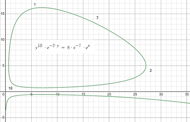
is called Lotka-Volterra system. E.g. let $a=10,b=2,c=7,d=1.$ Then we get the solution $y(t)^{10}\mathbf{e}^{-2y(t)}=\mathbf{e}^k x(t)^{-7}\mathbf{e}^{x(t)}.$

 

The Exponential Ansatz

We now look at the most simple differential equations and their solutions, linear ordinary ones over complex numbers
$$
y’=Ay\quad\text{ with a complex square matrix }A=(a_{ij})\in \mathbb{M}(n,\mathbb{C})
$$
A complex function
$$
y(t)=c\cdot \mathbf{e}^{\lambda t}
$$
is a solution of this equation if and only if $\lambda$ is an eigenvalue of the matrix $A$ and $c$ is a corresponding eigenvector. If $A$ has $n$ linearly independent eigenvectors (this is the case, for example, if A has $n$ distinct eigenvalues), then the system obtained in this manner is a fundamental system of solutions.

The theorem holds in the real case, too, but one has to deal with the fact, that some eigenvalues might not be real, and complex solutions are usually not the ones we are interested in over real numbers. The real version of the theorem has to deal with those cases and is thus a bit more technical.

Let’s consider the Jordan normal form of a matrix. Then $y’=Jy$ becomes
$$
\begin{cases}
y_1’&=\lambda y_1+y_2\\ y_2’&=\lambda y_2+y_3\\
\vdots &\vdots\quad \vdots\\
y_{n-1}’&=\lambda y_{n-1}+y_n\\
y_n’&=\lambda y_n
\end{cases}
$$
This system can easily be solved by a backward substitution
$$
Y(t)=\begin{bmatrix}
\mathbf{e}^{\lambda t}&t\mathbf{e}^{\lambda t}&\frac{1}{2}t^2\mathbf{e}^{\lambda t}&\cdots&\frac{1}{(n-1)!}t^{n-1}\mathbf{e}^{\lambda t}\\
0&\mathbf{e}^{\lambda t}&t\mathbf{e}^{\lambda t}&\cdots&\frac{1}{(n-2)!}t^{n-2}\mathbf{e}^{\lambda t}\\
0&0&\mathbf{e}^{\lambda t}&\cdots&\frac{1}{(n-3)!}t^{n-3}\mathbf{e}^{\lambda t}\\
\vdots&\vdots&\vdots&\ddots&\vdots\\
0&0&0&\cdots&\mathbf{e}^{\lambda t}
\end{bmatrix}
$$
The series
$$
\mathbf{e}^{B}=I+B+\dfrac{B^2}{2!}+\dfrac{B^3}{3!}+\ldots
$$
converges absolutely for all $B$ so we get
$$
\left(\mathbf{e}^{At}\right)’=A\cdot \mathbf{e}^{At}
$$
and found a fundamental matrix for our differential equation system, namely
$$
Y(t)=\mathbf{e}^{At}\quad \text{with}\quad Y(0)=I
$$

 

An important generalization in physics is periodic functions. Say we have a harmonic, $\omega$-periodic system with a continuous $A(t)$
$$
x'(t)=A(t)x(t)\quad\text{with}\quad A(t+\omega )=A(t)
$$
For it’s fundamental matrix $X(t)$ with $X(0)=I$ holds
$$
X(t+\omega )=X(t)C\quad\text{with a non-singular matrix}\quad C=X(\omega )
$$
$C$ can be written as $\mathbf{e}^{\omega B}$ although the matrix $B$ is not uniquely determined because of the complex periodicity of the exponential function.

Theorem of Gaston Floquet (1847-1920)

$X(t)$ with $X(0)=I$ has a Floquet representation
$$
X(t)=Q(t)\mathbf{e}^{ B t}
$$
where $Q(t)\in \mathcal{C}^1(\mathbb{R})$ is $\omega$-periodic and non-singular for all $t.$

 

Let us finally consider a more sophisticated, nevertheless important example: Lie groups. They occur as symmetry groups of differential equations in physics. A Lie group is an analytical manifold and an algebraic group. Its tangent space at the $I$-component is its corresponding Lie algebra. The latter can also be analytically introduced as left-invariant (or right-invariant) vector fields. The connection between the two is simple: differentiate on the manifold (Lie group) and you get to the tangent space (Lie algebra), integrate along the vector fields (Lie algebra), and you get to the manifold (Lie group).

The Lie Derivative

“Let $X$ be a vector field on a manifold $M$. We are often interested in how certain geometric objects on $M$, such as functions, differential forms and other vector fields, vary under the flow $\exp(\varepsilon X)$ induced by $X$. The Lie derivative of such an object will in effect tell us its infinitesimal change when acted on by the flow. … More generally, let $\sigma$ be a differential form or vector field defined over $M$. Given a point $p\in M$, after ‘time’ $\varepsilon$ it has moved to
$\exp(\varepsilon X)$ with its original value at $p$. However, $\left. \sigma \right|_{\exp(\varepsilon X)p}$ and $\left. \sigma \right|_p$, as they stand are, strictly speaking, incomparable as they belong to different vector spaces, e.g. $\left. TM \right|_{\exp(\varepsilon X)p}$ and $\left. TM \right|_p$ in the case of a vector field. To effect any comparison, we need to ‘transport’ $\left. \sigma \right|_{\exp(\varepsilon X)p}$ back to $p$ in some natural way, and then make our comparison. For vector fields, this natural transport is the inverse differential
\begin{equation*}
\phi^*_\varepsilon \equiv d \exp(-\varepsilon X) : \left. TM \right|_{\exp(\varepsilon X)p} \rightarrow \left. TM \right|_p
\end{equation*}
whereas for differential forms we use the pullback map
\begin{equation*}
\phi^*_\varepsilon \equiv \exp(\varepsilon X)^* : \wedge^k \left. T^*M \right|_{\exp(\varepsilon X)p} \rightarrow \wedge^k \left. T^*M \right|_p
\end{equation*}
This allows us to make the general definition of a Lie derivative.” [Olver]

The exponential function comes into play here, because the exponential map is the natural function that transports objects of the Lie algebra $\mathfrak{g}$ to those on the manifold $G$, a form of integration. It is the same reason we used the exponential Ansatz above since differential equations are statements about vector fields. If two matrices $A,B$ commute, then we have
$$
\text{addition in the Lie algebra }\longleftarrow \mathbf{e}^{A+B}=\mathbf{e}^{A}\cdot \mathbf{e}^{B}\longrightarrow
\text{ multiplication in the Lie group}
$$
The usual case of non-commuting matrices is a lot more complicated, however, the principle stands, the conversion of multiplication to addition and vice versa. E.g., conditions of the multiplicative determinant ($\det U = 1$) for the (unitary) Lie group turns into a condition of the additive trace ($\operatorname{tr}S=0$) for the (skew-Hermitian) Lie algebra.

The Lie derivative along a vector field $X$ of a vector field or differential form $\omega$ at a point $p \in M$ is given by
\begin{equation*}
\begin{aligned}
\mathcal{L}_X(\omega)_p &= X(\omega)|_p \\ &= \lim_{t \to 0} \frac{1}{t} \left( \phi^*_t (\left. \omega \right|_{\exp(t X)_p})- \omega|_p \right) \\
&= \left. \frac{d}{dt} \right|_{t=0}\, \phi^*_t (\left. \omega \right|_{\exp(t X)_p})
\end{aligned}
\end{equation*}
In this form, it is obvious that the Lie derivative is a directional derivative and another form of the equation we started with.

 

Both, Lie groups and Lie algebras have a so-called adjoint representation denoted by $\operatorname{Ad}\, , \,\mathfrak{ad},$ resp. Inner automorphisms (conjugation) on the group level become inner derivations (linear maps that obey the Leibniz rule in general, and the Jacobi identity in particular) on the Lie algebra level. Let $\iota_y$ denote the group conjugation $x\longmapsto yxy^{-1}.$ Then the derivative at the point $I$ is the adjoint representation of the Lie group (on its Lie algebra as representation space)
$$
D_I(\iota_y)=\operatorname{Ad}(y)\, : \,X\longmapsto yXy^{-1}
$$
The adjoint representation $\mathfrak{ad}$ of the Lie algebra on itself as representation space is the left-multiplication $(\mathfrak{ad}(X))(Y)=[X,Y].$ Both are related by
$$
\operatorname{Ad}(\mathbf{e}^A) = \mathbf{e}^{\mathfrak{ad} A}
$$

Sources