Creating and recovering a frequency shift in time domain in MATLAB

[tworitdash]

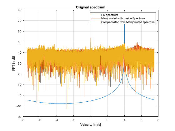
I am trying to simulate and process the Doppler signals. My main problem is a little more complex so I am only posting a simple version of it. Task1: I have a time-domain signal with the velocity of the target as mu. I need to change the velocity to mu cos(theta) where theta is a vector from 0 to 2 pi with the same number of points that I have in the time domain signal. So, every point in the original time-domain signal should have this change. This means that the Doppler frequency (velocity) is not constant with time. Task2: Then, after I get this signal, I want to recover the original spectrum (with constant velocity) but without knowing mu. I just need to know the phase and then modify it somehow to get the real signal.

 clear;
    close all;
    
    lambda = 0.03;
    M = 61;
    hs = 128;
    
    N = hs * M; % Number of points in the time axis
    
    mu = 4; % Doppler velocity
    
    
    PRT = 1e-3;  % Time step
    
    t1 = 0:PRT:(N - 1)*PRT; % Time axis
    
    
    s_ = exp(1j .* 4 * pi ./ lambda .* mu .* t1); % Original Time domain signal
    
    s_f = fftshift(fft(s_)); % FT of the original time domain signal
    
    v_amb = 7.5;
    
    v_axis = linspace(-N/2, N/2-1, N)/N .* 2 * v_amb; % Velocity axis
    
    figure; plot(v_axis, db(abs(s_f))); title('Original spectrum') % Original spectrum
    %% Task1:
    BW = 1*pi/180;
    p0 = 0*pi/180;
    p1 = 360*pi/180;
    th = linspace(p0, p1, N); % Angle axis for cos(theta)
    
    
    s_man_ = abs(s_) .* exp(1j .* (angle(s_)) + 1j * 4*pi/lambda * mu * (cos(th) - 1) .* t1); % Modified time domain signal with cos(theta)
    
    s_man_f_full = fftshift(fft(s_man_)); % FT of the modified time domain signal
    
    %% Task 2
    
    s_man_comp = abs(s_man_) .* exp(1j .* (angle(s_man_)) ./ cos(th)); % Reconstruction of the original signal in time domain
    
    s_man_comp_f = fftshift(fft(s_man_comp)); % FT of the reconstructed signal
    
    figure(1); hold on; plot(v_axis, db(abs(s_man_f_full)));
    
    hold on; plot(v_axis, db(abs(s_man_comp_f)));
    
    legend({'HD spectrum', 'Manipulated with cosine Spectrum', 'Compensated from Manipulated spectrum'});  grid on;

The figure is shown below. The Yellow plot should resemble the blue blot but it doesn't. Any idea what I do wrong here? The red plot also should show multiple spikes in the plot and not like a noise signal like this I suppose.

 

[NateD]

It looks like you are not correctly modifying the signal with the cosine theta vector. The theta vector should be used to modify the phase of the signal, not its amplitude. Try modifying the signal with a phase shift equal to mu * (cos(theta) - 1) * t1 and see if you get the desired results.