theblazierbroom
- 9
- 1
- Homework Statement
- A particle of mass m moves along a straight line. Its motion is resisted by a force proportional to its velocity, F=-k*v. It starts with speed v = v_0 at x = 0 and t = 0.
(a) Find x as a function of t by numerical integration.
(b) Find the time t_1/2 required to lose half its speed, and the maximum distance x_max attained.
Notes:
(1) Adjust the scales of x and t so that the equation of motion has simple numerical coefficients.
(2) Invent a scheme to attain good accuracy with a relatively coarse interval for delta t.
(3) Use dimensional analysis to deduce how t_1/2 and x_max should depend upon v_0, k, and m, and solve for the actual motion only for a single convenient value of v_0, say v_0 = 1.00 (in modified x and t units).
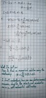
- Relevant Equations
- x(t_n) = \sum{i=0}^{n}{v(t_i)} * delta t
v(t_n) = \sum{i=0}^{n}{a(t_i)} * delta t
When I used differential equation techniques, I found the function of x and v to be a negative exponential function.
However, based on the notes, I believe the problem wants me to use finite summations as the relevant equations above. This stumps me because the acceleration is dependent on the velocity, and I get stuck in this self-referential thought process.
I believe figuring out a solution to this problem would help me better understand the thought process behind integration. I would appreciate any guidance!