Thorra
- 45
- 0
Hello! I have a nifty set of problems (or rather one problem, gradually building itself to be a great problem) that I like to collectively call "The final problem" as it is the last thing I need before I can take the exam in Numerical Methods.Information
There is given a Laplace equation $\frac{\partial^2 u}{\partial x^2} + \frac{\partial^2 u}{\partial y^2} = 0$ in a quadratic-type area $R = {(x,y)|0<x<1;0<y<1}$ with Neuman and Robin type boundary conditions $u(x,0)=0$ ; $\frac{\partial u(x,1)}{\partial y}+\frac{2u(x,1)}{(1+x^2)+1} = \frac{1}{(1+x^2)+1}$ ; $u(0,y)=\frac{y}{1+y^2}$ ; $\frac{\partial u(1,y)}{\partial x} = - \frac{4y}{(4+y^2)^2}$ .
Problem's analytical solution is $u(x,y)=\frac{y}{1+x^2)+y^2}$.
Tasks to do:
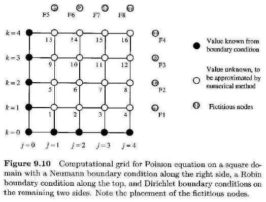
1. Approximate (with 2nd approximation order) the equation on the lattice/model with an even step ($h$ and $g$) in each of the directions $x$ and $y$, splitting each of the intervals $0<x<1$; $0<y<1$ in according parts $N$ and $M$.
2. Approximate (with 2nd approximation order) the given boundary conditions. For Neuman and Robin boundary conditions use fictive "nodal points" outside the area.
Okay... This is actually just the tip of the iceberg (apparently later I'll have to do programming... haha) but I already have trouble with this.
So I guess the 1st one I've kinda done before. I think it's something like:
$$\frac{u(x+h,y)-2u(x,y)+u(x-h,y)}{h^2}+\frac{u(x,y+g)-2u(x,y)+u(x,y-g)}{g^2}=0$$
where I $h$ and $g$ are divided into N and M parts $h=\frac{1}{N}$ and $g=\frac{1}{M}$ (1 being the interval length).
Errors are the old $\psi=\mathcal O(h^2+g^2)$.Now the 2nd one is a little trickier to me.
I counted 4 boundary conditions. Started with this one:
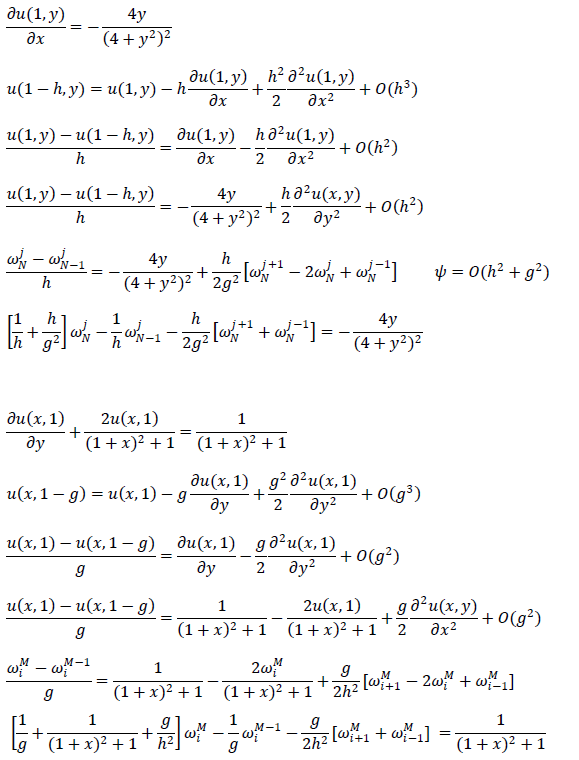
$$\frac{\partial u(1,y)}{\partial x}=-\frac{4y}{(4+y^2)^2}$$
I did this off a very similar example, but still not sure about it and not comprehending everything.
$$u(1+h,y)=u(1,y) + h\frac{\partial u(1,y)}{\partial x} + \frac{h^2}{2}\frac{\partial^2 u(1,y)}{\partial x^2} + O(h^3)$$
So that's just the ol' Taylor formula with the twist of taking the end point of x and stepping out of the model (this is what I naively interpret as the "fictive nodal point". It says to only use them on "Neuman" and "Robin" boundaries, but I don't think there even are any other boundary conditions).
Next we do the approximation of a first order derivative:
$$\frac{u(1+h,y)-u(1,y)}{h}=\frac{\partial u(1,y)}{\partial x}+\frac{h}{2}\frac{\partial^2 u(1,y)}{\partial x^2}+\mathcal O(h^2)$$
And now a really confusing moment for me:
$$\frac{u(1+h,y)-u(1,y)}{h}=-\frac{4y}{(4+y^2)^2}-\frac{h}{2}\frac{\partial^2 u(x,y)}{\partial y^2}+\mathcal O(h^2)$$
It's not the small substitution at the first part. It's the 2nd part where the u(1,y) magically turns into u(x,y) and x^2 turns into y^2. I just don't understand why would that be. It basically means that $$\frac{\partial^2 u(1,y)}{\partial x^2}=-\frac{\partial^2 u(x,y)}{\partial y^2}$$Thanks in advance.
There is given a Laplace equation $\frac{\partial^2 u}{\partial x^2} + \frac{\partial^2 u}{\partial y^2} = 0$ in a quadratic-type area $R = {(x,y)|0<x<1;0<y<1}$ with Neuman and Robin type boundary conditions $u(x,0)=0$ ; $\frac{\partial u(x,1)}{\partial y}+\frac{2u(x,1)}{(1+x^2)+1} = \frac{1}{(1+x^2)+1}$ ; $u(0,y)=\frac{y}{1+y^2}$ ; $\frac{\partial u(1,y)}{\partial x} = - \frac{4y}{(4+y^2)^2}$ .
Problem's analytical solution is $u(x,y)=\frac{y}{1+x^2)+y^2}$.
Tasks to do:
1. Approximate (with 2nd approximation order) the equation on the lattice/model with an even step ($h$ and $g$) in each of the directions $x$ and $y$, splitting each of the intervals $0<x<1$; $0<y<1$ in according parts $N$ and $M$.
2. Approximate (with 2nd approximation order) the given boundary conditions. For Neuman and Robin boundary conditions use fictive "nodal points" outside the area.
Okay... This is actually just the tip of the iceberg (apparently later I'll have to do programming... haha) but I already have trouble with this.
So I guess the 1st one I've kinda done before. I think it's something like:
$$\frac{u(x+h,y)-2u(x,y)+u(x-h,y)}{h^2}+\frac{u(x,y+g)-2u(x,y)+u(x,y-g)}{g^2}=0$$
where I $h$ and $g$ are divided into N and M parts $h=\frac{1}{N}$ and $g=\frac{1}{M}$ (1 being the interval length).
Errors are the old $\psi=\mathcal O(h^2+g^2)$.Now the 2nd one is a little trickier to me.
I counted 4 boundary conditions. Started with this one:
$$\frac{\partial u(1,y)}{\partial x}=-\frac{4y}{(4+y^2)^2}$$
I did this off a very similar example, but still not sure about it and not comprehending everything.
$$u(1+h,y)=u(1,y) + h\frac{\partial u(1,y)}{\partial x} + \frac{h^2}{2}\frac{\partial^2 u(1,y)}{\partial x^2} + O(h^3)$$
So that's just the ol' Taylor formula with the twist of taking the end point of x and stepping out of the model (this is what I naively interpret as the "fictive nodal point". It says to only use them on "Neuman" and "Robin" boundaries, but I don't think there even are any other boundary conditions).
Next we do the approximation of a first order derivative:
$$\frac{u(1+h,y)-u(1,y)}{h}=\frac{\partial u(1,y)}{\partial x}+\frac{h}{2}\frac{\partial^2 u(1,y)}{\partial x^2}+\mathcal O(h^2)$$
And now a really confusing moment for me:
$$\frac{u(1+h,y)-u(1,y)}{h}=-\frac{4y}{(4+y^2)^2}-\frac{h}{2}\frac{\partial^2 u(x,y)}{\partial y^2}+\mathcal O(h^2)$$
It's not the small substitution at the first part. It's the 2nd part where the u(1,y) magically turns into u(x,y) and x^2 turns into y^2. I just don't understand why would that be. It basically means that $$\frac{\partial^2 u(1,y)}{\partial x^2}=-\frac{\partial^2 u(x,y)}{\partial y^2}$$Thanks in advance.