- #1
- 1,598
- 605
- TL;DR Summary
- How does the number of electrons affect the boson or fermion nature of ions
In the theory of superfluidity, ##^{4}##He atoms are seen as weakly interacting pointlike bosons, with an integer total spin. Does a ##^3##He atom also become a boson if I add or remove one electron to give ##^3##He##^+## or ##^3##He##^-## ?
I'm trying to calculate the ground state wave functions of systems of two ions in a 2D or 3D potential well similar to those in this thread. The diffusion monte carlo code can't properly antisymmetrize a fermion system so I have to choose ions with an integer spin. I also assume that in this case most of the interaction is from the total charge on each ion and not from Van der Waals forces and the like.
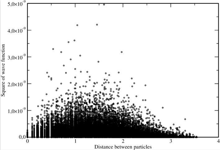
I already did one calculation for two fictitious particles with charge ##+2e## and mass ##m_e## in a 2D square potential well of depth ##V=1500## and side length ##L=3.0##. The program gives an output file with 5 columns that contain the two coordinates of each particle and the value of the wave function. Converting this to a 2-column file with first column containing interparticle distance and the second one containing the square of the wave function, a scatter plot with no connecting lines between data points looks like this:

This looks much like I expected, and a radial distribution function like ##P(r) = c_0 re^{-c_1 r} + c_2##, with the ##c_k## constants, can be fitted in this data to capture the main features.
I'm trying to calculate the ground state wave functions of systems of two ions in a 2D or 3D potential well similar to those in this thread. The diffusion monte carlo code can't properly antisymmetrize a fermion system so I have to choose ions with an integer spin. I also assume that in this case most of the interaction is from the total charge on each ion and not from Van der Waals forces and the like.
I already did one calculation for two fictitious particles with charge ##+2e## and mass ##m_e## in a 2D square potential well of depth ##V=1500## and side length ##L=3.0##. The program gives an output file with 5 columns that contain the two coordinates of each particle and the value of the wave function. Converting this to a 2-column file with first column containing interparticle distance and the second one containing the square of the wave function, a scatter plot with no connecting lines between data points looks like this:
This looks much like I expected, and a radial distribution function like ##P(r) = c_0 re^{-c_1 r} + c_2##, with the ##c_k## constants, can be fitted in this data to capture the main features.