Ensemble vs. time averages and Ashcroft and Mermin Problem 1.1

In summary, the probability of no collision in a given time interval can be calculated by breaking the interval into smaller intervals and using the product of the probabilities of no collision in each subinterval. This holds for both preceding and future time intervals due to the symmetry of time. Additionally, the probability of the time interval between collisions of an electron being t is equivalent to the probability of an electron having collided at t and colliding again between t and t+dt. This can be calculated using the independence of different time intervals and the probabilities from Drude Axiom 4. The calculation for parts (c), (d), and (e) may involve a different random variable, but the overall process is similar.
  • #1
EE18
112
13
Homework Statement
Please see the attached photo.
Relevant Equations
See below.
The question is as seen below:
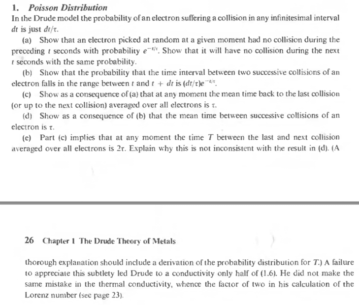
Screen Shot 2023-04-10 at 1.44.48 PM.png


My attempt (note that my questions are in bold below) is below. Please note that I am self-studying AM:

(a) By the independence of any interval ##dt## of time and time symmetry, we expect these two answers are the same (Is there any way to make this rigorous?). Divide the interval ##[0,t]## into ##N## intervals. Then the probability of no collision in ##[0,t]## is equal to the probability that there is no collision in each and every interval ##[t_i,t_i+t/N]##. Since each interval is statistically independent, we compute this probability (which we call ##P_{nc}(t)##) as the product of the probability of no collision in each interval, each of which is of length ##t/N## (i.e. these are i.i.d. intervals):
$$
P_{nc}(t) \equiv \lim_{n \to \infty} \left(1 - \frac{t}{N\tau}\right)^N = e^{-t/\tau}.
$$
We emphasize again that this is the probability that a given electron has not collided over the previous time ##t##, which is the same probability as that given electron not colliding over the future time ##t##.

(b)
The probability of the event that the time interval between collisions of an electron is ##t## can be argued (It's not clear to me why this should be the same as the probability that a given electron -- not necessarily just collided -- has time ##t## between two of its collisions.) to be the same as the probability of an electron which has just collided colliding again between ##t## and ##t+dt##. But this latter event is precisely the event ##A## that the electron does not collide in ##[0,t]## and ##B## also does collide in ##[t,t+dt)##. ##P(A)## is known from a), while ##P(B) = dt/\tau## from Drude Axiom 4. Thus, by the independence of different time intervals, we have ##P(A\&B) = P(A)P(B) = P_{nc}(t)dt/\tau = e^{-t/\tau}dt/\tau.##

For (c), (d), and (e), I am at a bit of a loss. I have read somewhere that I cannot seem to find now that perhaps this has something to do with the difference between an ensemble vs. time average, but it seems to me like what's really going on is that there is a different random variable under investigation in (c) and (d).
 
Physics news on Phys.org
  • #2
EE18 said:
My attempt (note that my questions are in bold below) is below. Please note that I am self-studying AM:

(a) By the independence of any interval ##dt## of time and time symmetry, we expect these two answers are the same (Is there any way to make this rigorous?). Divide the interval ##[0,t]## into ##N## intervals. Then the probability of no collision in ##[0,t]## is equal to the probability that there is no collision in each and every interval ##[t_i,t_i+t/N]##. Since each interval is statistically independent, we compute this probability (which we call ##P_{nc}(t)##) as the product of the probability of no collision in each interval, each of which is of length ##t/N## (i.e. these are i.i.d. intervals):
$$
P_{nc}(t) \equiv \lim_{n \to \infty} \left(1 - \frac{t}{N\tau}\right)^N = e^{-t/\tau}.
$$
We emphasize again that this is the probability that a given electron has not collided over the previous time ##t##, which is the same probability as that given electron not colliding over the future time ##t##.
This looks good to me.

The reason we expect the same result for the preceding ##t## seconds and for the next ##t## seconds is that the calculations for the two cases are essentially identical. For the preceding ##t## seconds, you would work with the time interval ##[-t, 0]##; for the future ##t## seconds, you work with the interval ##[0, t]##. Either way, you can break the interval into N subintervals and proceed as you did. So, unless I’m overlooking something, it should be clear that the probability of no collision during the preceding ##t## seconds should equal the probability of no collision during the next ##t## seconds.

EE18 said:
(b)
The probability of the event that the time interval between collisions of an electron is ##t## can be argued (It's not clear to me why this should be the same as the probability that a given electron -- not necessarily just collided -- has time ##t## between two of its collisions.) to be the same as the probability of an electron which has just collided colliding again between ##t## and ##t+dt##. But this latter event is precisely the event ##A## that the electron does not collide in ##[0,t]## and ##B## also does collide in ##[t,t+dt)##. ##P(A)## is known from a), while ##P(B) = dt/\tau## from Drude Axiom 4. Thus, by the independence of different time intervals, we have ##P(A\&B) = P(A)P(B) = P_{nc}(t)dt/\tau = e^{-t/\tau}dt/\tau.##
Again, this looks good. I’m not sure I understand your bold-faced concern. For part (b), I don’t see why you are concerned with an electron "not necessarily just collided”.

EE18 said:
For (c), (d), and (e), I am at a bit of a loss.
For part (c) you are picking an arbitrary instant of time which we can call the “present time”. Then, for each electron, there is a time interval ##t## from the present time to the electron’s next collision. The values of ##t## for the different electrons will be distributed with some probability distribution ##P(t)## such that ##P(t)dt## is the probability that the time interval from the present time to the next collision lies between ##t## and ##t+dt##. Using part (a) and using reasoning similar to that used in part (b), you can find an explicit expression for ##P(t)##. Then you can use ##P(t)## to find ##\langle t \rangle##, where ##\langle t \rangle## is the time interval between the present time and the next collision averaged over all the electrons.

Similarly, you can find the average time back to the previous collision.
 

FAQ: Ensemble vs. time averages and Ashcroft and Mermin Problem 1.1

What is the difference between ensemble averages and time averages?

Ensemble averages are statistical averages taken over a large number of identical systems at a single point in time, whereas time averages are taken over a single system over a long period of time. In equilibrium statistical mechanics, these two averages are often assumed to be equal, a hypothesis known as ergodicity.

Why is the concept of ergodicity important in statistical mechanics?

Ergodicity is crucial because it allows us to replace time averages, which can be difficult to compute, with ensemble averages, which are often easier to handle mathematically. This simplification is fundamental for connecting macroscopic thermodynamic properties with microscopic statistical properties.

What is the main focus of Ashcroft and Mermin Problem 1.1?

Ashcroft and Mermin Problem 1.1 typically introduces basic concepts of statistical mechanics and solid-state physics. The problem often involves understanding the behavior of particles in a system and calculating relevant statistical properties, such as distribution functions or averages.

How do you approach solving Ashcroft and Mermin Problem 1.1?

To solve Ashcroft and Mermin Problem 1.1, you should first clearly understand the physical scenario presented. Identify the relevant statistical quantities, apply appropriate statistical mechanics principles, and use mathematical techniques to derive the required results. Reviewing the underlying theory in the textbook can also provide valuable insights.

Can you provide a simple example illustrating the difference between ensemble and time averages?

Consider a simple system of a single particle in a box. For the time average, you would track the particle's position over a long period and calculate the average position. For the ensemble average, you would take a snapshot of many identical boxes, each with one particle, and calculate the average position of particles across all boxes at that instant. If the system is ergodic, these two averages should be the same.

Similar threads

Replies
1
Views
2K
Replies
1
Views
12K
Replies
1
Views
3K
Replies
6
Views
2K
Replies
1
Views
1K
Replies
17
Views
2K
Back
Top