Good values for gravitational potential

[fab13]

In the context of a project, I had to solve numerically Poisson equation with cylindrical coordinates. I put here results for z = 0 on a 3D mesh 256x256x256.

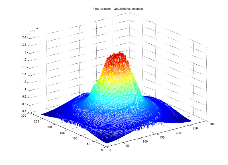
Below 1 figure representing the final solution (in absolute value) in the case of a galaxy; I use the CGS units for the potential.

I have 2 questions :

1*) I would like to know if the values that I get are valid with a similar real galaxy.

The characteristic features of this galaxy are : there are 10240 stars (each has 1 solar mass), the radius is equal to 25 kiloparsec (including arms).

A simple computation is done with the following formula :

abs(Phi(r)) = ∑ -Gm/(r-r(i))

For example, taking the positions of all the stars (10240 stars), I get for the potential at r = 1 kpc :

abs(Phi(1)) = 2.1 * 10^9 cm^2 s^-2

As you can see, I don't succeed to get the same value : look at near the center, I get approximately 2.5 10^12 cm^2 s^-2 : the difference is about 10^3, that's high.

Anyone could tell me why I don't get the same value for this radius ( r= 1 kpc) ?
In my code, I solve Poisson equation with discrete Fourier transform. Firstly, I compute the matter distribution (rho in Poisson equation) and after, the green function.

Here the code snippet for density (with space_x, space_y, space_y the size of a cell in grid, expressed in kiloparsec) :

for (i=0; i< Ng; i++)
  {
  for (j=0; j< Ng; j++)
  {
  for (k=0; k< Ng; k++)
  {
  compute(i, j, k, node_x, node_y, node_z); // Compute the coordinates of cell on the grid

  density[node_x][node_y][node_z] = density[node_x][node_y][node_z] + mass/((space_x*space_y*space_z));
  }
}
}

Here the code snippet for green function (with Ng=256 in my case) :

for (i=0; i< Ng; i++)
  {
  for (j=0; j< Ng; j++)
  {
  for (k=0; k< Ng; k++)
  {
  compute(i, j, k, node_x, node_y, node_z); // Compute the coordinates of cell on the grid
  density[node_x][node_y][node_z] = density[node_x][node_y][node_z] + mass/((space_x*space_y*space_z));
  }
}
}

2*) When I define Green function, have I to add a factor space_x, space_y and space_z respectively for dx, dy, dz ? I mean like this below :

for (i=0; i< Ng; i++)
  {
  for (j=0; j< Ng; j++)
  {
  for (k=0; k< Ng; k++)
  {
  compute(i, j, k, node_x, node_y, node_z); // Compute the coordinates of cell on the grid
  density[node_x][node_y][node_z] = density[node_x][node_y][node_z] + mass/((space_x*space_y*space_z));
  }
}
}

If I don't add these factors, i.e :

for (i=0; i< Ng; i++)
  {
  for (j=0; j< Ng; j++)
  {
  for (k=0; k< Ng; k++)
  {
  compute(i, j, k, node_x, node_y, node_z); // Compute the coordinates of cell on the grid
  density[node_x][node_y][node_z] = density[node_x][node_y][node_z] + mass/((space_x*space_y*space_z));
  }
}
}

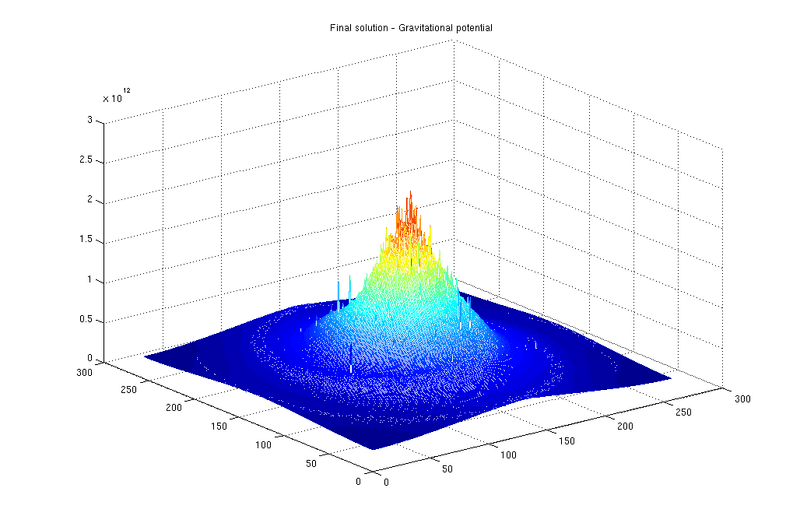
I get the following result :

As you can see, the potential is more smoothed around the center. So I don't know if I have to include or not these space_x, space_y and space_z in Green function.

From your experience and the characteristics of this galaxy (number of stars equal to 10240, solar mass for each star and radius about 25 kpc), which figure seems to be valid ? the first image or the second ?

Any help is welcome

 

[mfb]

You write about cylindrical coordinates but the code seems to use cartesian coordinates.

Apart from an empty line, where is the difference between the code snippets?
Also, how do you use that code? Where does "mass" come from?

If the stars have discrete positions you can get a massive spike for every star, especially if your grid point is close to a star. And I think that's what the plot is showing.

 

[fab13]

Sorry, I have forgotten to put the two good snippet codes (for the computing of Green's function) which corresponds respectively to the first and second plot :

figure 1 :

for (i=0; i< Ng; i++)
   {
    for (j=0; j< Ng; j++)
       {
        for (k=0; k< Ng; k++)
           {
             dx = sqrt(pow((double) (i-Ng/2),2.0))*space_x;
             dy = sqrt(pow((double) (j-Ng/2),2.0))*space_y;
             dz = sqrt(pow((double) (k-Ng/2),2.0))*space_z;
             green_grid[i][j][k] = -1.0/(4.0*M_PI*sqrt(dx*dx + dy*dy + dz*dz));
            }
       }
    }

figure 2 :

for (i=0; i< Ng; i++)
   {
    for (j=0; j< Ng; j++)
       {
        for (k=0; k< Ng; k++)
           {
             dx = sqrt(pow((double) (i-Ng/2),2.0));
             dy = sqrt(pow((double) (j-Ng/2),2.0));
             dz = sqrt(pow((double) (k-Ng/2),2.0));
             green_grid[i][j][k] = -1.0/(4.0*M_PI*sqrt(dx*dx + dy*dy + dz*dz));
            }
       }
    }

The differences between the 2 code snippets are the factors space_x, space_y and space_z (which are the size of a cell on the grid).

In my code, I compute firstly the discretized density with cartesian coordinates on a grid, then I compute the discretized Green's function on the same grid. After I apply a forward FFT for both, make their product and apply a backward FFT to get the discretized gravitational potential.

mass is equal to the solar mass ( = 2.0 10^33 g), I take for every star a mass equal to a solar mass.

My issue is so as I said :

As you can see, the potential is more smoothed around the center. So I don't know if I have to include or not these space_x, space_y and space_z in Green function.

 

[mfb]

Use fabs for absolute values, squaring (even worse: squaring with pow) and then taking the square root is more complicated and takes much more time.

Without context, I don't understand what that code is doing.

 

[fab13]

ok, in order to make you understand my issue, here's a Matlab sample code which reproduces my results :

clear;

G=6.67428*10^-8; %% cm^3 g^-1 s^-2
kpc=3.085678*10^21; %% 1kpc = 3.08 10^21 cm
mass=2.0*10^33; %% 1 solar mass = 2 10^33 g
factor_fft = 1.989*10^43;

data=load('Positions_Disk.dat');

% Number of star coordinates : 10240 with Positions_Disk.dat
numStars=numel(data(:,1));

% Number of r values
numPoints=numStars;

% Vector for r ccordinate
r=linspace(0,max(data(:,1)),numPoints);

%% Direct computing of gravitational potential
for i=1:numPoints
   Phi=0.0;
   for j=1:numStars
      Phi=Phi-G*mass/(abs(r(i)-sqrt(data(j,1)*data(j,1)+data(j,2)*data(j,2)+data(j,3)*data(j,3)))*kpc);
   end
   Value(i)=abs(Phi);
end

% For nice plot, delete spikes
for i=1:numPoints
    if Value(i) > 4*10^9
        Value(i) = 0.0
    end
end   

figure(1);
plot(r,Value);

%%% Solving Poisson equation with FFT

%% Compute the spacing of all cells
Ng=256;
Max_x=max(data(:,1));
Min_x=min(data(:,1));

Max_y=max(data(:,2));
Min_y=min(data(:,2));

Max_z=max(data(:,3));
Min_z=min(data(:,3));

if (Max_x>abs(Min_x))
  space_x=Max_x/(Ng/2);
  add_correction_x=-1;
else
  space_x=abs(Min_x)/(Ng/2);
  add_correction_x=0;
end

if (Max_y>abs(Min_y))
  space_y=Max_y/(Ng/2);
  add_correction_y=-1;
else
  space_y=abs(Min_y)/(Ng/2);
  add_correction_y=0;
end

if (Max_z>abs(Min_z))
  space_z=Max_z/(Ng/2);
  add_correction_z=-1;
else
  space_z=abs(Min_z)/(Ng/2);
  add_correction_z=0;
end

%% Computing coordinates on the grid
for i=1:numStars
    x(i)=data(i,1)/space_x + (Ng/2+add_correction_x);
    y(i)=data(i,2)/space_y + (Ng/2+add_correction_y);
    z(i)=data(i,3)/space_z + (Ng/2+add_correction_z);
end

density(1:Ng,1:Ng,1:Ng)=0.0;
green_grid(1:Ng,1:Ng,1:Ng)=0.0;

%% Computing the density for each cell
for i=1:numStars
  
    node_x = floor(x(i))+1;
    node_y = floor(y(i))+1;
    node_z = floor(z(i))+1;
  
    density(node_x,node_y,node_z) = density(node_x,node_y,node_z) + mass/(factor_fft*(space_x*space_y*space_z));

end
%% Computing discretized Green's function
for i=1:Ng
   for j=1:Ng
      for k=1:Ng
        
         %% First solution  : with space_x, space_y and space_z factors
         dx = sqrt((i-Ng/2)*(i-Ng/2))*space_x;
         dy = sqrt((j-Ng/2)*(j-Ng/2))*space_y;
         dz = sqrt((k-Ng/2)*(k-Ng/2))*space_z;
       
         %% Second solution : without space_x, space_y and space_z factors
         %dx = sqrt((i-Ng/2)*(i-Ng/2));
         %dy = sqrt((j-Ng/2)*(j-Ng/2));
         %dz = sqrt((k-Ng/2)*(k-Ng/2));
       
         green_grid(i,j,k) = -1.0/(4.0*pi*sqrt(dx*dx + dy*dy + dz*dz));

      end
   end
end

%% For avoiding divergence at Ng/2
green_grid(Ng/2,Ng/2,Ng/2) = 1.0;

%% FFT of Green
fft_green=fftn(green_grid);

%% FFT of density
fft_density=fftn(density);

%% Product in Fourier space
product_fft=4*pi*G*fft_green.*fft_density*factor_fft/kpc;

%% Backward of product above
fft_potential=real(ifftn(product_fft));

%% Shift final solution
fft_potential_shift=fftshift(fft_potential);

%% Mesh (1:256,1:256)
[x1 y1]=meshgrid(1:Ng,1:Ng);

%% Plot of potential (absolute value)
figure(2);
surf(x1,y1,abs(fft_potential_shift(:,:,Ng/2)));

As you can see, I am first computing the gravitational potential as a function of radius (the first figure). This is for getting an estimation of the potential with my data file "Positions_Disk.dat" which contains 3 columns (x,y,z coordinates of the stars) and 10240 lines.

After that, I solve the Poisson equation with discrete Fourier transform.

My problem is that I don't know if I have to add the factors space_x, space_y and space_z when I compute the discretized Green's function (

In all cases, I notice there's a big difference of values between the direct calculation of potential :

and the computation with fft :

You can see there is a difference on 10^3 between the 2 computations.

Anyone could help me to find which solution is valid ?

 

[mfb]

Phi=Phi-G*mass/(abs(r(i)-sqrt(data(j,1)*data(j,1)+data(j,2)*data(j,2)+data(j,3)*data(j,3)))*kpc);

I don't understand that line. You calculate the distance of the star to the origin (the sqrt term), and subtract that distance from r(i)? That does not give the distance between two points. Also, what is that r(i)?

For nice plot, delete spikes

Not surprising that you don't get larger values if you remove them manually.

 

[fab13]

I don't understand that line. You calculate the distance of the star to the origin (the sqrt term), and subtract that distance from r(i)? That does not give the distance between two points. Also, what is that r(i)?

r(i) corresponds to the distance between the origin and the point where I want to calculate the value of gravitational potential.

The gravitational potential at the point $$\vec{x_0}$$ of a collection of $$n$$ point objects of mass $$M_i$$ each located at a point $$\vec{x_i}$$ is: $$\begin{align} \Phi = \Sigma_{i=1}^{n} \frac{-GM_i}{|\vec{x_i}-\vec{x_0}|} \end{align}$$

Which solution do you suggest ?

 

[mfb]

You calculate $| |\vec{x_i}| - |\vec{x_0}| |$.
The subtraction has to be done with each component. sqrt( (r(i)_x - data(j,1))^2 + ... ) where (r(i)_x is the x-component of the (new) vector r(i).

 

[fab13]

ok, here below a new Matlab sample code which allows to do a direct computation of gravitational potential, i.e with :

$$\begin{align} \Phi = \Sigma_{i=1}^{n} \frac{-GM_i}{|\vec{x_i}-\vec{x_0}|} \end{align}$$

G=6.67428*10^-8; %% cm^3 g^-1 s^-2
kpc=3.085678*10^21; %% 1kpc = 3.08 10^21 cm
mass=2.0*10^33; %% 1 solar mass = 2 10^33 g

data=load('Positions_Disk.dat');

% Number of star coordinates : 10240 with Positions_Disk.dat
numStars=numel(data(:,1));

% Number of r values
numPoints=256;

% Vectors for x0, y0, z0 coordinates
x0=linspace(min(data(:,1)),max(data(:,1)),numPoints);
y0=linspace(min(data(:,2)),max(data(:,2)),numPoints);
z0=linspace(min(data(:,3)),max(data(:,3)),numPoints);

% Generating grid
[x y z]=meshgrid(x0,y0,z0);

%% Direct computing of gravitational potential
   for j=1:numPoints
      for k=1:numPoints
         for l=1:numPoints
            Phi(j,k,l)=0.0;
            for i=1:numStars
               Phi(j,k,l)=Phi(j,k,l)-G*mass/((sqrt((x(j,k,l)-data(i,1))^2+(y(j,k,l)-data(i,2))^2+(z(j,k,l)-data(i,3))^2))*kpc);
            end
            Value(j,k,l)=abs(Phi(j,k,l));
         end
      end
   end

% Plot potential for approximately z=0.0 kpc, i.e numPoints/2
figure(1);
surf(x(:,:,numPoints/2),y(:,:,numPoints/2),Value(:,:,numPoints/2));

I get with this script the following figure :

Unfortunately, I still have not the good values compared to the figure got with FFT computation, i.e this one :

As you can see on height coordinate, there is a 10^4 factor difference between the two figures.

How could I solve this problem of order of magnitude ? I should find similar values for the two computation.

Thanks

 

[mfb]

10^4 is the number of stars... some issue with the FFT normalization?

 

[fab13]

I don't think the issue comes from the FFT normalization because I use first a forward FFT and then a backward FFT.

I give you the Matlab sample code which achieves the solving by FFT :

G=6.67428*10^-8; %% cm^3 g^-1 s^-2
kpc=3.085678*10^21; %% 1kpc = 3.08 10^21 cm
mass=2.0*10^33; %% 1 solar mass = 2 10^33 g
factor_fft = 1.989*10^43;

data=load('Positions_Disk.dat');

%% Number of stars
numStars=numel(data(:,1));

%% Compute the spacing of all cells
Ng=256;
Max_x=max(data(:,1));
Min_x=min(data(:,1));

Max_y=max(data(:,2));
Min_y=min(data(:,2));

Max_z=max(data(:,3));
Min_z=min(data(:,3));

if (Max_x>abs(Min_x))
  space_x=Max_x/(Ng/2);
  add_correction_x=-1;
else
  space_x=abs(Min_x)/(Ng/2);
  add_correction_x=0;
end

if (Max_y>abs(Min_y))
  space_y=Max_y/(Ng/2);
  add_correction_y=-1;
else
  space_y=abs(Min_y)/(Ng/2);
  add_correction_y=0;
end

if (Max_z>abs(Min_z))
  space_z=Max_z/(Ng/2);
  add_correction_z=-1;
else
  space_z=abs(Min_z)/(Ng/2);
  add_correction_z=0;
end

%% Computing coordinates on the grid
for i=1:numStars
    x(i)=data(i,1)/space_x + (Ng/2+add_correction_x);
    y(i)=data(i,2)/space_y + (Ng/2+add_correction_y);
    z(i)=data(i,3)/space_z + (Ng/2+add_correction_z);
end

density(1:Ng,1:Ng,1:Ng)=0.0;
green_grid(1:Ng,1:Ng,1:Ng)=0.0;

%% Computing the density for each cell
for i=1:numStars
   
    node_x = floor(x(i))+1;
    node_y = floor(y(i))+1;
    node_z = floor(z(i))+1;
   
    density(node_x,node_y,node_z) = density(node_x,node_y,node_z) + mass/(factor_fft*(space_x*space_y*space_z));

end
%% Computing discretized Green's function
for i=1:Ng
   for j=1:Ng
      for k=1:Ng
         
         %% First solution  : with space_x, space_y and space_z factors
         dx = sqrt((i-Ng/2)*(i-Ng/2))*space_x;
         dy = sqrt((j-Ng/2)*(j-Ng/2))*space_y;
         dz = sqrt((k-Ng/2)*(k-Ng/2))*space_z;
        
         %% Second solution : without space_x, space_y and space_z factors
         %dx = sqrt((i-Ng/2)*(i-Ng/2));
         %dy = sqrt((j-Ng/2)*(j-Ng/2));
         %dz = sqrt((k-Ng/2)*(k-Ng/2));
        
         green_grid(i,j,k) = -1.0/(4.0*pi*sqrt(dx*dx + dy*dy + dz*dz));

      end
   end
end

%% For avoiding divergence at Ng/2
green_grid(Ng/2,Ng/2,Ng/2) = 1.0;

%% FFT of Green
fft_green=fftn(green_grid);

%% FFT of density
fft_density=fftn(density);

%% Product in Fourier space
product_fft=4*pi*G*fft_green.*fft_density*factor_fft/kpc;

%% Backward of product above
fft_potential=real(ifftn(product_fft));

%% Shift final solution
fft_potential_shift=fftshift(fft_potential);

%% Mesh (1:256,1:256)
[x1 y1]=meshgrid(1:Ng,1:Ng);

%% Plot of potential (absolute value)
figure(2);
surf(x1,y1,abs(fft_potential_shift(:,:,Ng/2)));

I think that issue could come from my computation of matter density, look at this computation :

  density(node_x,node_y,node_z) = density(node_x,node_y,node_z) + mass/(factor_fft*(space_x*space_y*space_z));

factor_fft is used to stay in the range of float type, I eliminate it in the product of density and Green FFTs.

Take a look at the definition of Green's function :

%% volume of a cell in kpc^3  : with space_x, space_y and space_z factors
         dx = sqrt((i-Ng/2)*(i-Ng/2))*space_x;
         dy = sqrt((j-Ng/2)*(j-Ng/2))*space_y;
         dz = sqrt((k-Ng/2)*(k-Ng/2))*space_z;

green_grid(i,j,k) = -1.0/(4.0*pi*sqrt(dx*dx + dy*dy + dz*dz));

and finally, I made the product of both FFT (just before the backward FFT) :

%% Product in Fourier space
product_fft=4*pi*G*fft_green.*fft_density*factor_fft/kpc; % I eliminate the factor_fft used above

I think problem is that I don't know how handle the CGS units.

Green's Function has here centimeter^⁻1 unit. The Fourier transform of Green's function is centimeter^2, isn't it ? ( FFT(-1/(4*pi*r) = -1/k^2))

But by the definition of Discrete Fourier transform, should'nt FFT of Green's function units are null ? Because

$$FFT(Green)(k) = \int Green(x)e^{-j2\pi kx} dx$$ ([dx] = centimeter and [Green(x)] = centimeter^-1

If anyone could explain me the dimensional units of these terms ...

 

[fab13]

I come back to you for solving my issue.

From the definition of Green's function which is the solution of :

$$\nabla^{2}G(x) = \delta(x)$$

I realized that units of Green's function are [distance], i.e a length because $$\int\delta(x) dx=1$$ and so delta function has [distance^-1] unit.

The problem is that Green function is defined by :

$$G(r) = -\dfrac{1}{4\pi r}$$

and from this form, we may think that Green function has the unit of [distance]^-1 because $$r$$ has [distance] unit, but this is in contradiction with above.

How to deal with this paradox ? In my case, I am solving Poisson's equation numerically with Fourier transform and I need to discretize the Green's function on a grid. My main issue is that I am working in CGS units, so I define the Green's function on the [Ng,Ng,Ng] grid by :

%% 1kpc = 3.08 10^21 cm
kpc=3.085678*10^21

%% Computing discretized Green's function
for i=1:Ng
  for j=1:Ng
  for k=1:Ng

%% First solution  : with space_x, space_y and space_z factors (x,y,z size of a cell on the grid in kiloparsec)
  %dx = sqrt((i-Ng/2)*(i-Ng/2))*space_x*kpc;
  %dy = sqrt((j-Ng/2)*(j-Ng/2))*space_y*kpc;
  %dz = sqrt((k-Ng/2)*(k-Ng/2))*space_z*kpc;%% Second solution : without space_x, space_y and space_z factors and kpc factors
  dx = sqrt((i-Ng/2)*(i-Ng/2));
  dy = sqrt((j-Ng/2)*(j-Ng/2));
  dz = sqrt((k-Ng/2)*(k-Ng/2));
  %% Units of Green's function : kpc
  green_grid(i,j,k) = -1.0/(4.0*pi*sqrt(dx*dx + dy*dy + dz*dz));

  end
  end
end

space_x*kpc

represents the side x size of each cell on the grid in centimeters

space_y*kpc

represents the side y size of each cell on the grid in centimeters

space_z*kpc

represents the side z size of each cell on the grid in centimeters

For example, when I take $$G(r=10 kpc) = -\dfrac{1}{4\pi 10}=-\dfrac{1}{40\pi}$$, have I got the same value than for $$G(r=10 cm)=-\dfrac{1}{4\pi 10}=-\dfrac{1}{40\pi}$$ ?

in others words, is Green's function independant from the units that we take when we want to compute it or have one to apply a factor as a function of units used ?

Thanks for your clarifications

 

[mfb]

G has units of inverse length. The second derivative of it is inverse distance cubed, or a "density". Integrate this density over a volume and you get a dimensionless value again.
You can multiply everything with a mass or other constants, but the length units work out nicely.

 

[fab13]

ok If I take G(r) unit as inverse length, How can I have [FT(G(r)] = length²

$$FT(G(r)) = \int G(r) e^{-j2\pi kr} dr = -\dfrac{1}{k^2}$$ knowing k unit is inverse length in frequency space ? so in my code :

Unit[FT(G(r)] = cm²

Moreover, delta function seems to have inverse length unit given this definition :

$$\int\delta(x) dx=1$$

Can you confirm this ? Maybe delta unit doesn't make sense.

Still with your suggestion, how could one have the potential unit equal to [distance^2][second^-2] knowing we can write the potential solution as :

$$\Phi(x) = 4\pi G \int G(x'-x)\,\rho(x') dx'$$ with :

1. [G] = g^-1.cm³.s^-2
2. [G(x-x')] = cm^-1
3. [\rho] = g.cm^-3
4. [dx'] = cm
   
5. So Finally, we would have : [\Phi(x)] = s^-2 which is not good

Thanks for your help

 

[mfb]

I lost track of the various formulas spread around in the thread, sorry.

 

[fab13]

Maybe I have a part of the solution for my issue. I have found the following paper which talks about the solving of poisson equation with Fourier transforms :

Link removed by mod per member request.

To match the notations I have used from the beginning of this thread, the factors $$h_{x}, h_{y}, h_{z}$$ in this paper correspond to $$space_{x}, space_{y}, space_{z}$$ in my question.

From this paper, it seems that I have to add $$h_{x}*h_{y}*h_{z}$$ factor to numerator of the discretized Green's function. They get this factor by calculating the Jacobian of the transformation :

$$(i,j,k) \rightarrow (x,y,z)$$

So It seems that I can calculate the Fourier transform of Green's function like this :

$$FT(G(r)) = FT(G(x,y,z))=\int G(r)e^{-j2\pi kr}dr = \int G(x,y,z)e^{-j2\pi k_{x}x+k_{y}y+k_{z}z}dxdydz$$

For my computing, I need to discretize this equation above. Can I write :

$$\hat{G}(r,s,t) = h_{x}h_{y}h_{z}\sum_{a}\sum_{b}\sum_{c}G(a,b,c)e^{-j2\pi( ra+sb+tc)/N}$$

$$\hat{G}(r,s,t) = space_{x}space_{y}space_{z}\sum_{a}\sum_{b}\sum_{c}G(a,b,c)e^{-j2\pi( ra+sb+tc)/N}$$

with

$$G(a,b,c)= -space_{x}space_{y}space_{z}/(4\pi *sqrt((space_{x}*(Ng/2-a)^2+space_{y}*(Ng/2-b)^2+space_{z}*(Ng/2-c)^2)))$$

and N the number of points for each dimension of the grid (which is equal to

Ng

in my code) ?

Moreover, in order to stay in CGS units and more precisely in $$[centimeters]units$$ for Green's function, have I got to replace in my code the three terms $$h_{x}, h_{y}, h_{z}$$ from the above paper by these terms :

hx=space_{x}*kpc
hy=space_{y}*kpc
hz=space_{z}*kpc

where kpc is the value of one kiloparsec expressed in centimeters ?

Thanks for your help