Hard MVT theorem proof Tutorial Q7

[TanWu]

Homework Statement

Throughout this Tutorial Q6 to Q9 let $c: \mathbb{R} \rightarrow \mathbb{R}$ be a differentiable function whose derivative $c^{\prime}$ is continuous at 0 with $c^{\prime}(0)=1$.

Relevant Equations

$c^{\prime}(0)=1$

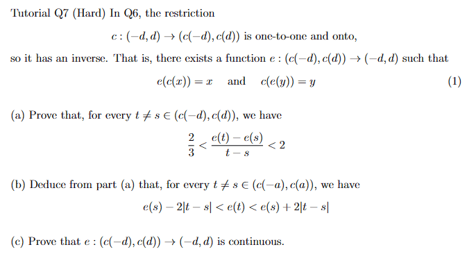
The tutorial question I am working on is,

(a) Attempt
We can use mean value theorem since

$(c: \mathbb{R} \rightarrow \mathbb{R}~countinity ) \implies (c: [-d, d] \rightarrow [c(-d), c(d)]~countinity)$

Thus $c: [-d, d] \rightarrow [c(-d), c(d)]$ is differentiable on $(-d, d)$, then there exists $b \in (-d, d)$ such that $c'(b) = \frac{c(-d) - c(d)}{-d - d} = \frac{f(-d) - f(d)}{-2d}$

Using result from Q6,
$b \in (-d, d) \implies \frac{1}{2} < \frac{f(-d) - f(d)}{-2d} < \frac{3}{2}$

Not sure how to prove from here.

(b) Attempt
$\frac{2}{3}(t - s) < e(t) - e(s) < 2(t - s)$
$\frac{2}{3}(t - s) + e(s) < e(t) < 2(t - s) + e(s)$

However, this is far from the expression that I am trying to prove.

(c) Nothing yet (may rely on (a) and (b))

I express gratitude to those who help

 

[Mark44]

Using result from Q6, $b \in (-d, d) \implies \frac{1}{2} < \frac{f(-d) - f(d)}{-2d} < \frac{3}{2}$

How did you arrive at this inequality? You don't show Q6, so it's hard to tell where it comes from.
Also, it doesn't seem that you have used the given information that f'(0) = 1.

 

[TanWu]

How did you arrive at this inequality? You don't show Q6, so it's hard to tell where it comes from.
Also, it doesn't seem that you have used the given information that f'(0) = 1.

Thank you Sir. My apologies the Q6 I posted is awaiting approval. There was a typo, it is meant to be c'(0) = 1. (The derivative of the function c at 0). The result I am using is from Q6.

 

[Office_Shredder]

You can use the chain rule to express the derivative of e in terms of the derivative of c. This lets you put bounds on the derivative of e. Try starting with that and then see how the mean value theorem helps

 

[nuuskur]

Please avoid using some ambiguous word soup as a title. None of us know what Hard or Medium hard means and which Q7 of which tutorial it is. The only helpful part of the title currently is "MVT".

 

[TanWu]

You can use the chain rule to express the derivative of e in terms of the derivative of c. This lets you put bounds on the derivative of e. Try starting with that and then see how the mean value theorem helps

Please avoid using some ambiguous word soup as a title. None of us know what Hard or Medium hard means and which Q7 of which tutorial it is. The only helpful part of the title currently is "MVT".

Both sir thank you.

Using your hint,

$(a)$
Let $e(t) = x$ and $e(s) = y$, and we perform change of variables for the definition of inverse function.
Thus $e(c(v)) = v$ and $c(e(w)) = w$

Thus,

$e(c(v)) = v$ and $e(t) = x$ imply $t = c(v)$ and $x = v$ which then imply $t = c(x)$

$e(c(v)) = v$ and $e(s) = y$ imply $s = c(v)$ and $y = v$ which then imply $s = c(y)$

Now we find difference quotient for inverse function, we call this difference quotient a speical name the MVT. $e(t)$:

$\frac{e(t) - e(s)}{t - s} = \frac{x - y}{c(x) - c(y)} = \frac{1}{\frac{c(x) - c(y)}{x - y}} = \frac{1}{c'(z)}$ where since this a difference quotient, $x < z < y$

Then using for all $z \in (-d,d)$, we have $\frac{1}{2} < c'(z) < \frac{3}{2}$

Then inverting the inequality,

$\frac{1}{\frac{1}{2}} > \frac{1}{c'(z)} > \frac{1}{\frac{3}{2}}$

$2 > \frac{1}{c'(z)} > \frac{2}{3}$

$\frac{2}{3} < \frac{e(t) - e(s)}{t - s} < 2$

QED.

Whew, That is a tiresome proof.

 

[TanWu]

(b)

$\frac{2}{3} < \frac{e(t) - e(s)}{t - s} < 2 \implies \frac{e(t) - e(s)}{t - s} < 2$

Then take absolute value of each side,

$\frac{|e(t) - e(s)|}{|t - s|} < |2|$

Which is equivalent to

$\frac{|e(t) - e(s)|}{|t - s|} < 2$

With some rearrangement, we get

$-2|t - s| + e(s) < e(t) < 2|t - s| + e(s)$

QED.

 

[TanWu]

For $(c)$,

For $e(c(-d), c(d)) \rightarrow (-d,d)$ to be continuous, it must be right continuous at $c(d)$ and left hand continuous at $c(-d)$ and uniformly continuous on $(-d,d)$.

That is, $\lim_{t \rightarrow [c(- d)^+]} e(t) = e(c(-d))= -d$ and $\lim_{t \rightarrow [c(d)^-]} e(t) = e(c(d))= d$ from the definition of e as the inverse of c on $(-d,d)$.

To prove that uniform continuity on $t \in (c(-d), c(d))$, since we know that, $|e(t) - e(s)| < 2|t - s|$ this implies that $|e(t) - e(s)| \le C|t - s|$ where $c < 2 \in \mathbb{R}$.

Take $C = 1.5$ Then $|e(t) - e(s)| \le 1.5|t - s|$ thus e is lipschitz continuous and thus continuous on the interval as required. QED.

I assume if no one replies my proof is correct for (a) and (c) which I still have slight doubts about.

 

[Office_Shredder]

If e is a function from $(-c(d),c(d))\to \mathbb{R}$ then since the domain is an open interval the endpoints aren't in the domain. Hence proving it's continuous at the endpoints makes no sense - the function isn't even defined at those points

 

[TanWu]

If e is a function from $(-c(d),c(d))\to \mathbb{R}$ then since the domain is an open interval the endpoints aren't in the domain. Hence proving it's continuous at the endpoints makes no sense - the function isn't even defined at those points

Thank you Sir that is a good point, I forgot that right/left continuity is only for half closed/open interval or closed interval. So one only needs lipschitz continuity to prove uniform continuity in this instance. Do you know of any other ways to prove uniform continuity without using lipschitz continuity since I have not really studied that yet much.

 

[Office_Shredder]

I agree that this function is uniformly continuous, but you said it "must" be uniformly continuous and it's not true that continuous functions are uniformly continuous on open intervals in general.

But I do think the thing you did is correct. No need for word salad with different forms of continuity - it's continuous at s because for any epsilon if $|s-t|<\epsilon/2$ then $|e(s)-e(t)|<\epsilon$

 

[TanWu]

I agree that this function is uniformly continuous, but you said it "must" be uniformly continuous and it's not true that continuous functions are uniformly continuous on open intervals in general.

But I do think the thing you did is correct. No need for word salad with different forms of continuity - it's continuous at s because for any epsilon if $|s-t|<\epsilon/2$ then $|e(s)-e(t)|<\epsilon$

Thank you Sir. Would you know why you set $|s-t|<\epsilon/2$. I mean like why use $\epsilon/2$ instead of $\delta$? It is because for continuity and limit proofs $\delta \le \epsilon$ so you were just expressing $\delta(\epsilon )$ (Delta as a function of epsilon)?

 

[Office_Shredder]

Thank you Sir. Would you know why you set $|s-t|<\epsilon/2$. I mean like why use $\epsilon/2$ instead of $\delta$? It is because for continuity and limit proofs $\delta \le \epsilon$ so you were just expressing $\delta(\epsilon )$ (Delta as a function of epsilon)?

I was expressing $\delta$ as a function of $\epsilon$.

It is not true that $\delta \leq \epsilon$ in general