How Accurate is Numerical Differentiation of sin(x) at 0.4?

In summary: And h is not plotted on a log scale.)The black curve in post #7 is the correct plot: it is the error ##|f_{num}(0.4,h)-(-sin(0.4))|\ ## against h (on a log scale). As you can see for yourself, it starts at the correct value ##10^{-3}## (for k = 1, as I am lazy and like Excel) and then rises as h decreases until it gets overwhelmed by the double precision issue. So your plot is not right, but you have done a lot of work and are close. Look again at the values in post #9 and what I did with them in post #7.I don't have
  • #1
roam
1,271
12
I am trying to estimate the second derivative of ##sin(x)## at ##0.4## for ##h=10^{-k}, \ \ k=1, 2, ..., 20## using:

$$\frac{f(x+h)-2f(x)+f(x-h)}{h^2}, \ \ (1)$$

I know the exact value has to be ##f''(0.4)=-sin(0.4)= -0.389418342308651.##

I also want to plot the error as a function ##h## in Matlab.

According to my textbook equation (1) has error give by ##h^2f^{(4)}/12##. So I am guessing ##f^{(4)}## refers to the fifth term in the Taylor expansion which we can find using Matlab syntax taylor(f,0.4):

sin(2/5) - (sin(2/5)*(x - 2/5)^2)/2 + (sin(2/5)*(x - 2/5)^4)/24 + cos(2/5)*(x - 2/5) - (cos(2/5)*(x - 2/5)^3)/6 + (cos(2/5)*(x - 2/5)^5)/120

So substituting this in, here is my code for ##f''(0.4)## and error so far:

Code:
format long
x=0.4;

for k = 1:1:20
    h=10.^(-k);
    ddf=(sin(x+h)-2*sin(x)+sin(x-h))./(h.^2)
    e=((h.^2)*((cos(2/5)*(x - 2/5).^3)/6))./12
     plot(h,e)
end

But this does not converge and I get some strange values for ##f''## which are very different from the exact value I found above:

Code:
ddf = -0.389093935175844
ddf = -0.389415097166723
ddf = -0.389418309876266
ddf = -0.389418342017223
ddf = -0.389418497448446
ddf = -0.389466237038505
ddf = -0.388578058618805
ddf = -0.555111512312578
ddf = 0.00
ddf = 0.00
ddf = -5.551115123125782e+05
ddf = 0.00
ddf = 0.00
ddf = 0.00
ddf = -5.551115123125782e+13
ddf = 0.00
ddf = 0.00
ddf = 0.00
ddf = 0.00
ddf = 0.00

What is wrong with my code? :confused:

And for the error I get all zeros, so it is not possible to plot error vs h. But I believe the graph should look something like this image:
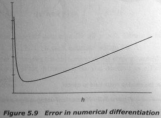
2016_03_19_19_15_33.jpg


So, what do I need to do here?

Any help would be greatly appreciated.
 
Physics news on Phys.org
  • #2
Hello roam,

what I see looks a lot like crossing the limits of what you can do with double precision: by the time ##h^2 < 10^{-15}## things go awry. Not in the denominator, but in the numerator.
 
  • Like
Likes roam
  • #3
Hi BvU,

Yes, that's true. Do you know by any chance why the error is always equal zero? Am I using the wrong formula or the wrong code?
 
Last edited:
  • #4
Formula is fine, code is fine too, but not usable for this purpose: the code is hampered by the selfsame issue you try to demonstrate. As far as I can find, Matlab always uses double precision (about 15 significant digits), so once the relative difference becomes too small, you get noise and then zero. Print sin(x-h), sin(x) and sin(x+h) to see it happen.

Study the way double precision numbers are stored to understand why this happens.

You could try to improve precision, but it will only help you a few steps further -- you'll need more than 80 digits of precision for your whole graph...
 
Last edited:
  • Like
Likes roam
  • #5
The reason the error is always equal to zero is that you are calculating it incorrectly. You have a function[itex]f_{num}(x,h)[/itex] that is calculating the derivative at x, given a value of h. To calculate the error, you should take:
[tex] abs(f_{num}(x,h) - f_{exact}(x))[/tex]
Your error term has a factor of (x-2/5) in it, and since x = 2/5, of course it gives zero. To calculate the predicted error correctly, the term [itex] f^{(4)}[/itex] refers to the 4th derivative of f, which in this case is sin(x), so the predicted error should be:
[tex] \frac{h^2 sin(0.4)}{12}[/tex]
It would be interesting to compare this predicted error with your calculated error as calculated above.
 
  • Like
Likes roam
  • #6
Phyz is correct, of course. (I wasn't looking any further than ddf -- where the results were already not as expected).

In fact the exercise can be done with excel comfortably as well and it gives the (Phyz) expected result -- up to k = 4 , so when ##h^4 = 10^{-16}##

upload_2016-3-20_23-14-53.png

Not unreasonable: we are subtracting ##\approx \cos(x+h/2)## from ## \approx \cos(x - h/2)##
 
  • Like
Likes roam
  • #7
Thank you very much Phyz, I have now managed to calculate ##e## correctly. The values seem reasonable when I compared them with the calculated error (as given by your equation).

Thank you BvU, I think your explanation is why the result seems very erratic, when you have a difference which is close enough to zero.

Anyway, I have now plotted the error function against ##h##:

error.jpg


er2.jpg


Is it about right? Would you say it looks anything like the generic shape of the error function as illustrated by the figure in my first post?
 
  • #8
I miss the upswing when h is close to zero. Don't you plot h < 0.001 ?

Code:
k   h         | sin(0.4) - ddif |
1 0.1          0.000324407
2 0.01         3.24514E-06
3 0.001        3.24324E-08
4 0.0001       2.91428E-10
5 0.00001      7.10251E-07
6 0.000001     4.78947E-05
7 0.0000001    0.000840284
8 0.00000001   0.16569317
 
  • #9
Why is that? I plotted all the values, here's are the values used:

Code:
e=[3.245152852572088e-04
3.245152852572088e-06
3.245152852572088e-08
3.245152852572088e-10
3.245152852572087e-12
3.245152852572088e-14
3.245152852572088e-16
3.245152852572088e-18
3.245152852572088e-20
3.245152852572088e-22
3.245152852572088e-24
3.245152852572088e-26
3.245152852572088e-28
3.245152852572088e-30
3.245152852572088e-32
3.245152852572087e-34
3.245152852572088e-36
3.245152852572088e-38
3.245152852572087e-40
3.245152852572088e-42];h=[0.100000000000000
    0.010000000000000
    1.000000000000000e-03
    1.000000000000000e-04
    9.999999999999999e-06
    1.000000000000000e-06
    1.000000000000000e-07
    1.000000000000000e-08
    1.000000000000000e-09
    1.000000000000000e-10
    1.000000000000000e-11
    1.000000000000000e-12
    1.000000000000000e-13
    1.000000000000000e-14
    1.000000000000000e-15
    1.000000000000000e-16
    9.999999999999999e-18
    1.000000000000000e-18
    1.000000000000000e-19
    1.000000000000000e-20];
 
  • #10
Looks like you plotted ##\
\frac{h^2 sin(0.4)}{12}\ ## ? That is not the error ! That's the predicted error !
 
  • Like
Likes roam

FAQ: How Accurate is Numerical Differentiation of sin(x) at 0.4?

What is numerical differentiation?

Numerical differentiation is a method used to estimate the derivative of a function at a particular point by using a finite difference approximation. It involves calculating the slope of a tangent line at a given point on a curve by taking the difference between two nearby points and dividing it by their distance.

Why is numerical differentiation important?

Numerical differentiation is important because it allows us to approximate the derivative of a function at a given point without having to know the exact mathematical formula for the function. This is useful in situations where the function is too complex or difficult to differentiate analytically, or when only a set of discrete data points are available.

What are the advantages of numerical differentiation over analytical differentiation?

One advantage of numerical differentiation is that it can be used for any function, regardless of its complexity or whether a closed-form solution exists. It also allows for more accurate results when dealing with functions that have a high degree of nonlinearity or contain discontinuities.

What are the different types of numerical differentiation?

The most commonly used types of numerical differentiation are forward, backward, and central difference methods. Forward difference uses the slope between a point and a point slightly to the right, backward difference uses the slope between a point and a point slightly to the left, and central difference uses the average of the slopes from both sides of a point.

What are the limitations of numerical differentiation?

Numerical differentiation is subject to rounding and truncation errors, which can affect the accuracy of the results. It also requires a small step size between data points to obtain more accurate results, which can be computationally expensive. Additionally, it may not work well for functions with sharp changes or discontinuities, as the slope between nearby points may not accurately represent the actual derivative at that point.

Similar threads

Replies
5
Views
2K
Replies
13
Views
2K
Replies
1
Views
2K
Replies
4
Views
2K
Replies
1
Views
814
Replies
11
Views
3K
Back
Top