How to Plot the Light Path in a Space-Time Diagram Using Python?

[AdrianD]

TL;DR Summary

Space-time diagram with python

I am trying to replicate the space time plot (the 2nd plot with Proper distance vs Time) as in this thread: space-time
I wrote everything in python using the astropy cosmology package.
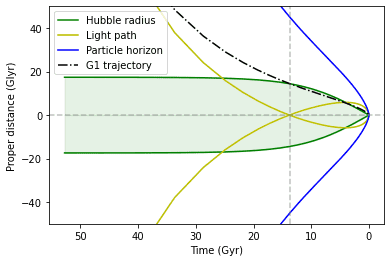
Everything went smooth, but I am stuck at plotting the light path on the 'purple path', as per the above example. I don't know how to plot the light path for the light emitted by the galaxy at t0 = 0 (now), with the proper distance of aprox 13.8 Glyr, that will reach us a t=49 Gyr.
Here is the code in python:

from astropy.cosmology import Planck18, z_at_value
from astropy import units as u
import numpy as np
from matplotlib import pyplot as plt
from scipy import interpolate as inter
import astropy.constants as cc# Hubble radius

def Hradius(zed):
    c = cc.c
    return (c/cosmo.H(zed)).to(u.Glyr)

#define cosmology

cosmo = Planck18
# Z and time

redshift = np.arange(-0.9,1089,0.1)

redshift_R = redshift[::-1]

time=cosmo.age(redshift)
# trajectory of a galaxy G1 with z=1.48

TrajectoryG1 = [cosmo.scale_factor(i) * cosmo.comoving_distance(1.48737).to(u.Glyr).value for i in redshift]
### Can't make it work

#lightPathG1 = [cosmo.scale_factor(0) * cosmo.comoving_distance(i).to(u.Glyr).value for i in redshiftG1]
# horizons

hubbleRadius = [Hradius(i).value for i in redshift]

hubbleRadiusMirrored = [-Hradius(i).value for i in redshift]

lightPath = [cosmo.scale_factor(i) * cosmo.comoving_distance(i).to(u.Glyr).value for i in redshift]

lightPathMirrored = [cosmo.scale_factor(i) * -cosmo.comoving_distance(i).to(u.Glyr).value for i in redshift]term1 = [cosmo.scale_factor(i) for i in redshift]

term2 = [cosmo.comoving_distance(i).to(u.Glyr).value for i in redshift_R]

term3 = [-cosmo.comoving_distance(i).to(u.Glyr).value for i in redshift_R]

particleHorizon = [term1*term2 for i in range(len(redshift))]

particleHorizonMirrored = [term1*term3 for i in range(len(redshift))]
#plot

fig, ax1 = plt.subplots()

ax1.plot(time,hubbleRadius, 'g-', label = 'Hubble radius')

ax1.plot(time,hubbleRadiusMirrored, 'g-')

ax1.plot(time,lightPath, 'y-', label = 'Light path')

ax1.plot(time,lightPathMirrored, 'y-')

ax1.plot(time,particleHorizon, 'b-', label = 'Particle horizon')

ax1.plot(time,particleHorizonMirrored, 'b-')
ax1.plot(time,TrajectoryG1, 'k',linestyle='-.', label = 'G1 trajectory')

#ax1.plot(timeG1,lightPathG1, color = 'orange')
ax1.set_ylim(ymin=-50, ymax=50)

ax1.axvline(x=13.7,color='grey',linestyle='--',alpha=0.5)

ax1.axhline(y=0,color='grey',linestyle='--',alpha=0.5)
ax1.fill_between(np.append(time.value, time[::-1].value), np.append(hubbleRadius, hubbleRadiusMirrored[::-1]), color = 'green', alpha = 0.1)
ax1.invert_xaxis()

ax1.legend()

ax1.set_xlabel('Time (Gyr)')

ax1.set_ylabel('Proper distance (Glyr)')

And my plot :