Material Model: initial conditions of equation?

[emadbeni]

Hello guys,

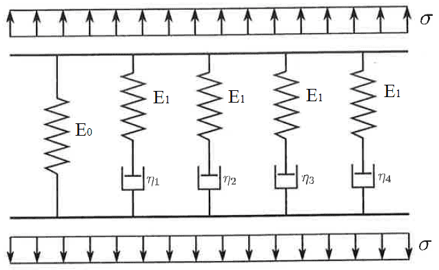
actually I'am working on a model to describe the creep-behaviour of a concrete specimen. This model is based on a 'generalized maxwell-chain'. I attached a picture, where you can see it:

The acting load is the tension $\sigma$, while $E_0$ and $E_1$ are the stiffnesses of the Hooke-springs and $\eta_i$ are the viscosities of the Newton-dashpots.

All these parameters are "hidden" in the parameters $a_i, b_i$ of the constitutive equation which describes the behaviour of this model by:

$b_0\cdot\epsilon+b_1\cdot\dot\epsilon+b_2\cdot\ddot\epsilon+b_3\cdot\dddot\epsilon + b_4\cdot\ddddot\epsilon = a_0\cdot\sigma +a_1\cdot\dot\sigma + a_2\cdot\ddot\sigma + a_3\cdot\dddot\sigma + a_4\cdot\ddddot\sigma$

To simplify the whole problem, I assume that these parameters $a_i, b_i$ won't change within time.

Now I want to test the material by performing a "simple" creep-test. This means that at a time $t$, a tension $\sigma > 0$ is applied and stays constant:

t = 0: σ = 0
t = 1: σ = 0
t = 2: σ = 0
t = 3: σ = 0
t = 3,001: σ = 1
t = 4: σ = 1
t = 5: σ = 1
t = 6: σ = 1
t = 7: σ = 1

(etc.)

If I want to know the resulting strain $\epsilon$ at the end of a time-step t-t0, i can solve the given equation which actually can be simplified to (because the $\sigma$ is constant in a time-step, all of it's derivatives are zero):

$b_0\cdot\epsilon+b_1\cdot\dot\epsilon+b_2\cdot\ddot\epsilon+b_3\cdot\dddot\epsilon + b_4\cdot\ddddot\epsilon = a_0\cdot\sigma$

This is a fourth-order ODE with constant coefficients that can be solved analytically. In a time-step based calculation, I have to solve the equation for each time-step by the formulation of correct initial conditions. ... and there is the problem:

If I want to get the strain et the end of the time step $(t = 3,001) - (t_0 = 3)$ I mean that the initial conditions for the $\epsilon, \dot\epsilon, ...$ are:

$\epsilon(t = 3) = 0 + \frac{\Delta\sigma(t-t_0)}{E_0 + 4\cdot E_1}$ (at the begin $\epsilon$ is zero, but there's always a kind of elastic deformation, when some stress is applied)
$\dot\epsilon(t = 3) = \frac{\frac{\Delta\sigma}{t - t_0}}{E_0 + 4\cdot E_1}$ (this is the velocity of the elastic strain)
$\ddot\epsilon(t = 3) = 0$ (I guess ... but I am not sure)
$\dddot\epsilon(t = 3) = 0$ (same here ...)

So far so good. If I come to the next time step $(t = 4) - (t_0 = 3,001)$, I have to solve the equation again. Now with different initial conditions:

$\epsilon(t = 4) = \epsilon(t = 3,001)+ \frac{\Delta\sigma(t-t_0) = 0}{E_0 + 4\cdot E_1}$
$\dot\epsilon(t = 4) = ...$ I don't know what... (I don't think that it is $\dot\epsilon(t = 3,001)$ and I also doubt that it is zero ...)
$\ddot\epsilon(t = 4) = ...$ (same here ...)
$\dddot\epsilon(t = 4) = ...$ (same here ...)

I hope I described the problem good enough that someone can help me ... this would be great!

Thank you in advance

 

[Chestermiller]

Hello guys,

actually I'am working on a model to describe the creep-behaviour of a concrete specimen. This model is based on a 'generalized maxwell-chain'. I attached a picture, where you can see it:

View attachment 78072

The acting load is the tension $\sigma$, while $E_0$ and $E_1$ are the stiffnesses of the Hooke-springs and $\eta_i$ are the viscosities of the Newton-dashpots.

All these parameters are "hidden" in the parameters $a_i, b_i$ of the constitutive equation which describes the behaviour of this model by:

$b_0\cdot\epsilon+b_1\cdot\dot\epsilon+b_2\cdot\ddot\epsilon+b_3\cdot\dddot\epsilon + b_4\cdot\ddddot\epsilon = a_0\cdot\sigma +a_1\cdot\dot\sigma + a_2\cdot\ddot\sigma + a_3\cdot\dddot\sigma + a_4\cdot\ddddot\sigma$

To simplify the whole problem, I assume that these parameters $a_i, b_i$ won't change within time.

Now I want to test the material by performing a "simple" creep-test. This means that at a time $t$, a tension $\sigma > 0$ is applied and stays constant:

t = 0: σ = 0
t = 1: σ = 0
t = 2: σ = 0
t = 3: σ = 0
t = 3,001: σ = 1
t = 4: σ = 1
t = 5: σ = 1
t = 6: σ = 1
t = 7: σ = 1

(etc.)

If I want to know the resulting strain $\epsilon$ at the end of a time-step t-t0, i can solve the given equation which actually can be simplified to (because the $\sigma$ is constant in a time-step, all of it's derivatives are zero):

$b_0\cdot\epsilon+b_1\cdot\dot\epsilon+b_2\cdot\ddot\epsilon+b_3\cdot\dddot\epsilon + b_4\cdot\ddddot\epsilon = a_0\cdot\sigma$

This is a fourth-order ODE with constant coefficients that can be solved analytically. In a time-step based calculation, I have to solve the equation for each time-step by the formulation of correct initial conditions. ... and there is the problem:

If I want to get the strain et the end of the time step $(t = 3,001) - (t_0 = 3)$ I mean that the initial conditions for the $\epsilon, \dot\epsilon, ...$ are:

$\epsilon(t = 3) = 0 + \frac{\Delta\sigma(t-t_0)}{E_0 + 4\cdot E_1}$ (at the begin $\epsilon$ is zero, but there's always a kind of elastic deformation, when some stress is applied)
$\dot\epsilon(t = 3) = \frac{\frac{\Delta\sigma}{t - t_0}}{E_0 + 4\cdot E_1}$ (this is the velocity of the elastic strain)
$\ddot\epsilon(t = 3) = 0$ (I guess ... but I am not sure)
$\dddot\epsilon(t = 3) = 0$ (same here ...)

So far so good. If I come to the next time step $(t = 4) - (t_0 = 3,001)$, I have to solve the equation again. Now with different initial conditions:

$\epsilon(t = 4) = \epsilon(t = 3,001)+ \frac{\Delta\sigma(t-t_0) = 0}{E_0 + 4\cdot E_1}$
$\dot\epsilon(t = 4) = ...$ I don't know what... (I don't think that it is $\dot\epsilon(t = 3,001)$ and I also doubt that it is zero ...)
$\ddot\epsilon(t = 4) = ...$ (same here ...)
$\dddot\epsilon(t = 4) = ...$ (same here ...)

I hope I described the problem good enough that someone can help me ... this would be great!

Thank you in advance

Do you have to solve it in the exact form of the differential equation you have written, or are other methods also acceptable?

Chet

 

[emadbeni]

Do you have to solve it in the exact form of the differential equation you have written, or are other methods also acceptable?

Chet

Hello Chet,
thanks a lot for your reply.

[unfortunately] I have to solve it (for each time-step) in the exact form (I just can move to numerical methods, if there's no way round) ...

this evening, I found an interesting script with some examples for rheological models in solid mechanics: http://homepages.engineering.auckla...sticity/10_Viscoelasticity_03_Rheological.pdf

On page 300, there's question "5.(c)" that gives maybe an hint how to deal with those initial conditions I am asking about. ... unfortunately I can't follow, how they found their condition in this (much simplier) example ...

I think that it might be possible to transform this solution somehow to my problem ... - unfortunately I don't know how to do this actually ...

emadbeni

 

[Chestermiller]

This is not how I would approach a problem like this. I think that trying to solve it analytically for the case of 5 elements present is daunting. The fact that they were able to solve it analytically with 2 elements present is very impressive.

I would approach this problem numerically, using the relaxation spectrum version 10.3.32. At each time step, I would put in a strain increment, and determine the corresponding stress increment. Then I would appropriately adjust the strain increment so that the stress increment comes out to be zero.

Of course, you could take the Laplace Transform of the relaxation spectrum version 10.3.32, and then solve for the Laplace Transform of the strain (for a step function stress). But being able to invert the resulting transform analytically would be a long shot.

Chet

 

[emadbeni]

... I see.

But, ... do you think that there exist an analytical solution for the problem? (Even if there are later on some stress-changes when there's a more complex creep-test performed?)

(Some weeks ago I tried it to solve the whole ODE by Laplace Transform; unfortunately this wasn't very practicable, because there turned out some real "bad" terms, where finding some partial fractions was not really possible ... - that's why I've choosen the way, to solve the given ODE by using a "classical" Ansatz. ... This works pretty well, the problem are as mentionned unfortunately "just" those bad initial-conditions for every time-step ... :/ )

 

[Chestermiller]

... I see.

But, ... do you think that there exist an analytical solution for the problem? (Even if there are later on some stress-changes when there's a more complex creep-test performed?)

I don't think so. I think that you already answered this question below when you tried to do it using Laplace Transforms, and the resolution into partial fractions became untractable. What you are really asking is "do I think the denominator of the Laplace Transform can be factored analytically?" I don't think so.

(Some weeks ago I tried it to solve the whole ODE by Laplace Transform; unfortunately this wasn't very practicable, because there turned out some real "bad" terms, where finding some partial fractions was not really possible ... - that's why I've choosen the way, to solve the given ODE by using a "classical" Ansatz. ... This works pretty well, the problem are as mentionned unfortunately "just" those bad initial-conditions for every time-step ... :/ )

 

[emadbeni]

What you are really asking is "do I think the denominator of the Laplace Transform can be factored analytically?" I don't think so.

That might be true ... yes.

Mhhm ... seems that I have to think over the whole procedure again ... But: there's one question remaining and maybe you have a hint for me. It's this "ominous" point "5.c." in this script I mentionned above. There it says (concerning the model which consists of two parallel maxwell units):

One initial condition results from the fact that only the springs react at time $$t = 0$$, which leads to the condition $$\epsilon(0) = \frac{\sigma_0}{E_1+E_2}$$. A second condition can be obtained by integrating the constitutive equation across $$t = 0$$ as in the footnote in §10.3.2. Show that this leads to the condition: $$\dot\epsilon(0^+) = \frac{\sigma_0}{t_R}\bigl[ \frac{\frac{\eta_1}{E_1}+\frac{\eta_2}{E_2}}{\eta_1+\eta_2} - \frac{1}{E_1+E_2}\bigr]$$ ... and $$t_R = \frac{\eta_1\cdot \eta_2}{\eta_1+\eta_2}\cdot\frac{E_1+E_2}{E_1\cdot E_2}$$.

I tried to do it in the same way that is described in this footnote.

For a model that consists of two parallel maxwell-units, the constitutive equation is given by:

$$\sigma+\frac{E_1\cdot\eta_1+E_2\cdot\eta_1}{E_1\cdot E_2}\cdot\dot\sigma + \frac{\eta_1\cdot\eta_2}{E_1\cdot E_2}\cdot\ddot\sigma = (\eta_1+\eta_2)\cdot\dot\epsilon + \frac{E_1+E_2}{E_1\cdot E_2}\eta_1\cdot \eta_2\ddot\epsilon$$

This equation simplifies, if we know that there acts just a constant tension $$\sigma_0$$ on the system ($$\sigma(t) = \sigma_0 = \text{const.}; \dot\sigma(t) = 0 = \ddot\sigma(t)$$):

$$\sigma_0 = (\eta_1+\eta_2)\cdot\dot\epsilon + \frac{E_1+E_2}{E_1\cdot E_2}\cdot\eta_1\eta_2\cdot\ddot\epsilon$$

Then I integrate this equation around the point of loading:

$$\int_{-\Delta\tau}^{+\Delta\tau}\sigma_0\text{d}t = (\eta_1+\eta_2)\cdot\int_{-\Delta\tau}^{+\Delta\tau}\dot\epsilon(t)\text{d}t + \frac{E_1+E_2}{E_1\cdot E_2}\eta_1\cdot\eta_2\cdot\int_{-\Delta\tau}^{+\Delta\tau}\ddot\epsilon(t)\text{d}t$$

Integrating leads to:

$$0 = (\eta_1 + \eta_2)\cdot [\epsilon(t+\Delta\tau) - \epsilon(t-\Delta\tau)] + \frac{E_1+E_2}{E_1\cdot E_2}\eta_1\cdot\eta_2\cdot [\dot\epsilon(t+\Delta\tau)-\dot\epsilon(t-\Delta\tau)]$$

Limits (and taking care about the fact there has been no initial strain [= on the "left side"] but there's this elastic jump in strain [= on the "right side"]) gives:

$$0 = (\eta_1+\eta_2)\cdot\frac{\sigma_0}{E_1+E_2} + \frac{E_1+E_2}{E_1\cdot E_2}\eta_1\cdot \eta_2\cdot \dot\epsilon(t)$$

... but that's not really the thing that should be shown as quoted above.

Where did I make the mistake? ... I don't get it ... :/

 

[Chestermiller]

That's not how I would integrate the equation, and that's now how to solve (basically) a first order linear ordinary differential in dε/dt. I would substitute z for dε/dt, and then use either the integrating factor method, or the method of separation of variables to solve for z. Then I would integrate that equation for z to determine ε. Try this approach, and see what you get.

Chet

 

[emadbeni]

So you mean, i should solve (with z = dε/dt):

$$\sigma_0 = (\eta_1+\eta_2)\cdot z + \frac{E_1+E_2}{E_1\cdot E_2}\cdot \eta_1\cdot\eta_2 \dot z$$

for z?! Why?

I can't really follow ... I've already solved the whole constitutive equation (seperately for the homogeneous and for the particular part); the problem is "just" finding the correct initial condition for $$\dot\epsilon(t = 0) = ...$$.

emad

 

[Chestermiller]

So you mean, i should solve (with z = dε/dt):

$$\sigma_0 = (\eta_1+\eta_2)\cdot z + \frac{E_1+E_2}{E_1\cdot E_2}\cdot \eta_1\cdot\eta_2 \dot z$$

for z?! Why?

I can't really follow ... I've already solved the whole constitutive equation (seperately for the homogeneous and for the particular part); the problem is "just" finding the correct initial condition for $$\dot\epsilon(t = 0) = ...$$.

emad

You need to go back to 10.3.29 and integrate across t = 0.

Chet

 

[emadbeni]

Uh ... that was it.
Now I got the solution ... unfortunately I am not sure, whether I really understood the background of this procedure (the 'why' to integrate the constitutive equation) as well as the things, I mentionned in the following:

The constitutive equation is:

$$\sigma + \frac{E_1\eta_2+E_2\eta_1}{E_1 E_2}\cdot\dot\sigma + \frac{\eta_1\eta_2}{E_1 E_2}\cdot\ddot\sigma = (\eta_1+\eta_2)\cdot\dot\epsilon +\frac{E_1+E_2}{E_1 E_2}\eta_1 \eta_2\cdot \ddot\epsilon$$

I now integrate across the point of loading (here it's t = 0):

$$\sigma\cdot\int_{-\Delta\tau}^{+\Delta\tau}\text{d}t + \frac{E_1\eta_2+E_2\eta_1}{E_1 E_2}\cdot \int_{-\Delta\tau}^{+\Delta\tau}\dot\sigma\text{d}t + \frac{\eta_1 \eta_2}{E_1 E_2}\cdot \int_{-\Delta\tau}^{+\Delta\tau}\ddot\sigma\text{d}t = (\eta_1+\eta_2)\cdot\int_{-\Delta\tau}^{+\Delta\tau}\dot\epsilon\text{d}t + \frac{E_1+E_2}{E_1 E_2}\eta_1\eta_2\cdot \int_{-\Delta\tau}^{+\Delta\tau}\ddot\epsilon\text{d}t$$

This gives (while thinking about Delta Tau --> 0

$$\underbrace{0}_{\text{turns into zero}} + \frac{E_1\eta_2 + E_2\eta_1}{E_1 E_2}\cdot\bigl[ \sigma(t+\Delta\tau)-\sigma(t-\Delta\tau)\bigr] + \underbrace{\frac{\eta_1\eta_2}{E_1 E_2}\cdot\bigl[ \dot\sigma(t+\Delta\tau)-\dot\sigma(t-\Delta\tau)\bigr]}_{\text{= 0, because we've a constant Load acting}} ==$$
$$==(\eta_1+\eta_2)\cdot\bigl[\underbrace{\epsilon(t+\Delta\tau)}_{=\frac{\sigma_0}{E_1+E_2}}-\underbrace{\epsilon(t-\Delta\tau)}_{= 0} \bigr] + \frac{E_1+E_2}{E_1\cdot E_2}\eta_1\eta_2\cdot\bigl[ \underbrace{\dot\epsilon(t+\Delta\tau)-\dot\epsilon(t-\Delta\tau)}_{=\dot\epsilon(t=0)}\bigr]$$

... and solving for depsilon/dt gives the solution of the script.

But ... is the statement in the last underbraced term correct? I imagine that I get as solution of the whole problem a moreless continuous curve and therefore, the derivative depsilon of epsilon in exact the point t=0 is the difference depsilon(t+Delta_t)-depsilon(t+Delta_t) ... (because depsilon+ is infitesimal bigger, and depsilon- infinitesimal smaller than depsilon we're looking for ...

emad

P.S.: Is this procedure 'universally valid'? I mean if I have - as an example - a model consisting of five maxwell-elements? (I know that it gets harder to handle, the bigger those models are ... but just for interest.)

 

[Chestermiller]

There is one part that I don't understand, and that's the part about the integral of the third term on the σ side of the equation. I don't see where that has to be zero. As far as your PS question is concerned, since we have been struggling even with the first couple of derivative terms, I can't imagine how it could possibly be applied to even more elements.

Chet

 

[emadbeni]

There is one part that I don't understand, and that's the part about the integral of the third term on the σ side of the equation. I don't see where that has to be zero.

I think that this could be explained. - If we perform the integration of the constitutive equation, we can do it ... somehow like a recipe. ... But, if we are about to let DeltaTau --> 0, we have to care about the values of the functions:
For the first term, we know that any sigma is a constant. Therefore sigma(t+DeltaT)-sigma(t-DeltaT) has to be zero.
For the second term, we know sigma at both sides (the function of sigma is a kind of "stepfunction" in this case): sigma(t+DeltaT) = sigma0 and sigma(t-DeltaT) = 0.
The third term contains the first derivative of the function of sigma which describes our loading. As the "function" sigma is zero at t-DeltaT, dsigma/dt at this point should also be zero, because there is no change of sigma here; after loading the system with sigma0, it stays constant. Because every constants derivatives are zero, we can say that dsigma/dt(t+DeltaT) is zero as well ...

Thats how I think about it ...

But finally, I have another "practical" question left: I tried to plot some diagrams of

$$\epsilon(t) = \sigma_0\cdot\biggl[\frac{1}{E_1+E_2}\cdot e^{\frac{-t}{t_R}}+\biggl(\frac{\frac{\eta_1}{E_1}+\frac{\eta_2}{E_2}}{\eta_1+\eta_2}-\frac{t_R}{\eta_1+\eta_2}\biggr)\cdot\biggl(1-e^{\frac{-t}{t_R}}\biggr)+\frac{t}{\eta_1+\eta_2}\biggr]$$
with
$$t_R = \frac{\eta_1\cdot \eta_2\cdot (E_1+E_2)}{(\eta_1+\eta_2)\cdot E_1\cdot E_2}$$

for

E1 = 1000
E2 = 1000
ƞ1 = 1500
ƞ2 = 100000

... in Excel. This works pretty well, if I take the equation and let Excel calculate epsilon(t) directly. ... In another case I now need an incremental/time-step formulation of this equation above. And now: nothing works ... - I don't know why. - Isn't it possible to formulate this given equation somehow like: epsilon(t) = epsilon(t_i-1)+epsilon(t_i).

Something in cell-form like (the italic epsilon(...) is the equation in time-step-form:

t = 0; sigma = 0; epsilon = 0
t = 1; sigma = 1; epsilon(t=1) = epsilon(t=1, t0)
t = 2; sigma = 1; epsilon(t=2) = epsilon(t=2, t1) + epsilon(t=1)
t = 3; sigma = 1; epsilon(t=3) = epsilon(t=3, t2) + epsilon(t=2)
t = i; sigma = 1; epsilon(t=i) = epsilon(t=i, ti-1) + epsilon(t=i)

... That would another great thing, if someone can help me here ...

emad

 

[Chestermiller]

I think that this could be explained. - If we perform the integration of the constitutive equation, we can do it ... somehow like a recipe. ... But, if we are about to let DeltaTau --> 0, we have to care about the values of the functions:
For the first term, we know that any sigma is a constant. Therefore sigma(t+DeltaT)-sigma(t-DeltaT) has to be zero.
For the second term, we know sigma at both sides (the function of sigma is a kind of "stepfunction" in this case): sigma(t+DeltaT) = sigma0 and sigma(t-DeltaT) = 0.
The third term contains the first derivative of the function of sigma which describes our loading. As the "function" sigma is zero at t-DeltaT, dsigma/dt at this point should also be zero, because there is no change of sigma here; after loading the system with sigma0, it stays constant. Because every constants derivatives are zero, we can say that dsigma/dt(t+DeltaT) is zero as well ...

I see what you are saying. That makes sense.

I wish I could have helped you out more on this, but I'm out of ideas.

Chet[/QUOTE]