Non quadratic potentials and quantization in QFT (home exercise)

[manfromearth]

Homework Statement

I'm given a field theory described by the lagrangian density
$$L=i\bar{\Psi}\gamma^{\mu}\partial_{\mu}\Psi-{{1}\over{2}}\partial_{\mu}\phi\partial^{\mu}\phi-g\phi\bar{\Psi}\Psi-{{\lambda}\over{4}}\phi^4+{{3m^2}\over{2}}\phi^2+{{2m^3}\over{\sqrt{\lambda}}}\phi$$


I'm asked to (1) find all the particles described by this theory, (2) find the Feynman rules and then (3) compute the differential cross section at tree level for the process $$\pi\pi\rightarrow\pi\pi$$, where $\pi$ is the particle described by excitations of $\phi$

Relevant Equations

I wrote the potential for the $\phi$ field as
$$V(\phi)={{\lambda}\over{4}}\phi^4-{{3m^2}\over{2}}\phi^2-{{2m^3}\over{\sqrt{\lambda}}}\phi$$

I noticed that $V(\phi)$ has nonzero minima, therefore I found the stationary points as ${{\partial{V}}\over{\partial\phi}}=0$, and found the solutions:
$$\phi^0_{1,2}=-{{m}\over{\sqrt{\lambda}}}\quad \phi^0_3={{2m}\over{\sqrt{\lambda}}}$$
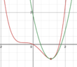
of these, only $\phi^0_3$ is a stable minimum, while the other two solutions are inflection points of $V$. (I attached a plot of such potential)

Now, I expect that expanding $V(\phi)$ around $\phi^0_3$ should give me the so called "mass spectrum" (because I was told so), so what I did was to approximate $V(\phi)$ around the minimum configuration and substitute such approximated potential in the lagrangian density $L$ as follows:

$$V(\phi)=V(\phi^0_3)+{{1}\over{2}}V^{\prime\prime}(\phi-\phi^0_3)^2+O(\Delta\phi^2)$$

dropping constant terms and higher orders, I found the approximated potential as:

$$V(\phi)={{9m^2}\over{2}}(\phi-{{2m}\over{\sqrt{\lambda}}})^2$$
Then, I defined a new field $\chi$ as the oscillation from the equilibrium position: $\chi=\phi-{{2m}\over{\lambda}}$ and by substituting $\chi$ in $L$ I found a new lagrangian in terms of the fields $\Psi$ and $\chi$:
$$\tilde{L}=\bar{\Psi}(i\gamma^{\mu}\partial_{\mu}-{{2mg}\over{\sqrt{\lambda}}})\Psi-{{1}\over{2}}(\partial_{\mu}\chi)^2-g\chi\bar{\Psi}\Psi-{{9m^2}\over{2}}\chi^2$$
So I conclude that this lagrangian describes a fermion field $\Psi$ of mass $m_{\Psi}=2mg/\sqrt{\lambda}$ and a neutral scalar particle $\chi$ of mass $m_{\chi}=3m$. The Feynman rules consist of those from Yukawa theory and come from the $g\chi\bar{\Psi}\Psi$ term.

This is where I get confused. Assuming that the $\pi$ particle is the one associated with the field $\chi$, the process $$\pi\pi\rightarrow\pi\pi$$ cannot be described at tree level using only Yukawa vertices. This makes me believe that I got the interaction terms wrong, and that I should not have expanded $V$, however I remember hearing something about "fields are just excitations around stable configurations" and "we can only quantize around the minimum" which was the initial motivation to do all of the above.

I guess my question is if it is always sensible to expand the potential at quadratic order, or if in doing so I loose interactions?
Am I missing something?

 

[AndreasC]

You don't need the Taylor expansion part. You get the masses by looking at the mass terms, ie the ones quadratic in fields. Where did you see that you have to do the Taylor expansion? Perhaps they didn't mean Taylor expansion but rather what you did with the χ field. After all doing a Taylor expansion doesn't make that much sense here, it is already a polynomial. Dropping terms will cost you interactions.