- #1
VVS
- 91
- 0
Hello,
I want to estimate a set of parameters by trying to minimize the sum of squares wrt to the parameter set given a simulation of a markov process and real data in Matlab. I have already implemented the Levenberg-Marquart (LM) Algorithm and it is converging to certain values and it is reasonably good.
But now I want to implement the Newton Raphson method, since it (should be) is more accurate. I don't care how long it will take. I am pretty sure that I am evaluating the Jacobian correctly since I am using it in the LM Algorithm. However I have doubts evaluating the Hessian Matrix:
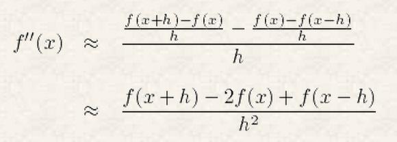
First, I approximately calculate the 2nd derivatives of my Simulation wrt to all parameters using the equation attached below as "2nd derivative approximation for diagonal elements" for diagonal elements and using the equation attached below as "2nd derivative approximation for off diagonal elements" for off diagonal elements.
To evaluate the derivatives I have to step the parameter values one by one (in this case by 1%) and simulate the model (see 2nd block of code). I am not sure whether I did this correctly. My second doubt about the Hessian is the first term given in the equation. We have to sum over i and multiply the residual by the Hessian matrix. The residual ri(theta) is a n x 1 vector where n is the number of data points and Hi(theta)is a p x p x n Matrix where p is the number of parameters. I am not sure if I have implemented this correctly in the code (see 1st block of code).
Hessian:

2nd derivative approximation for diagonal elements

2nd derivative approximation for off diagonal elements

The Algorithm
Evaluating h
Homework Statement
I want to estimate a set of parameters by trying to minimize the sum of squares wrt to the parameter set given a simulation of a markov process and real data in Matlab. I have already implemented the Levenberg-Marquart (LM) Algorithm and it is converging to certain values and it is reasonably good.
But now I want to implement the Newton Raphson method, since it (should be) is more accurate. I don't care how long it will take. I am pretty sure that I am evaluating the Jacobian correctly since I am using it in the LM Algorithm. However I have doubts evaluating the Hessian Matrix:
First, I approximately calculate the 2nd derivatives of my Simulation wrt to all parameters using the equation attached below as "2nd derivative approximation for diagonal elements" for diagonal elements and using the equation attached below as "2nd derivative approximation for off diagonal elements" for off diagonal elements.
To evaluate the derivatives I have to step the parameter values one by one (in this case by 1%) and simulate the model (see 2nd block of code). I am not sure whether I did this correctly. My second doubt about the Hessian is the first term given in the equation. We have to sum over i and multiply the residual by the Hessian matrix. The residual ri(theta) is a n x 1 vector where n is the number of data points and Hi(theta)is a p x p x n Matrix where p is the number of parameters. I am not sure if I have implemented this correctly in the code (see 1st block of code).
Homework Equations
Hessian:
2nd derivative approximation for diagonal elements
2nd derivative approximation for off diagonal elements
The Attempt at a Solution
The Algorithm
Code:
function [parameter_values]=Newton2

% load data to fit
data=load('WLMSR_Traces_Exp.mat');
Data_Current=data.WLMSR_10V;
Data_Time=data.time;

% initialize starting parameter values
alpha1 = 0.022348;
zalpha1 = 0.01176;
beta1 = 0.047002000000000002;
zbeta1 = -0.0631;
Kf = 0.023761000000000001;
Kb = 0.036777999999999998;
alpha2 = 0.013733;
zalpha2 = 0.038198;
beta2 = 6.8899999999999994e-005;
zbeta2 = -0.04178;

% initialize parameter names
parameter_values=[alpha1; zalpha1; beta1; zbeta1; Kf; Kb; alpha2; zalpha2; beta2; zbeta2];
parameter_names = cell(size(parameter_values));
parameter_names{1}='alpha1';
parameter_names{2}='zalpha1';
parameter_names{3}='beta1';
parameter_names{4}='zbeta1';
parameter_names{5}='Kf';
parameter_names{6}='Kb';
parameter_names{7}='alpha2';
parameter_names{8}='zalpha2';
parameter_names{9}='beta2';
parameter_names{10}='zbeta2';

% initialize file names
input_file_string='WLMSR_Model.txt';
output_file_string='WLMSR_Model_New.txt';
experiment_file_string='10.exp';

% initialize Simulation parameters
Simulation_Step_Time=2.5;
Simulation_Time=15000;
offset=5000;
subsampling_rate=3;

iterations=2;

for i=1:iterations

    fprintf('Iteration start time was\n');
    c = clock;
    disp(datestr(datenum(c(1),c(2),c(3),c(4),c(5),c(6))));


    [Simulation_Current_0] = Simulate1(input_file_string, output_file_string, parameter_names, parameter_values, experiment_file_string, Simulation_Step_Time, Simulation_Time, offset, subsampling_rate);

    residual=Data_Current-Simulation_Current_0;

    J = Evaluate_Jacobian(input_file_string, output_file_string, parameter_names, parameter_values, experiment_file_string, Simulation_Step_Time, Simulation_Time, offset, subsampling_rate);

    g = -2*transpose(J)*residual;

    % Compute Hessian Matrix

    [h] = Evaluate_h(input_file_string, output_file_string, parameter_names, parameter_values, experiment_file_string, Simulation_Step_Time, Simulation_Time, offset, subsampling_rate, Data_Current);

    H = 0;

    for j=1:length(residual)

        H = H + residual(j)* h(:,:,j);

    end

    H = -2*(H - transpose(J)*J);

    parameter_values = parameter_values - H\g

    fprintf('Iteration end time was\n');
    c = clock;
    disp(datestr(datenum(c(1),c(2),c(3),c(4),c(5),c(6))));

end
end
Evaluating h
Code:
function [h] = Evaluate_h(input_file_string, output_file_string, parameter_names, parameter_values, experiment_file_string, Simulation_Step_Time, Simulation_Time, offset, subsampling_rate, Data_Current)

for i=1:length(parameter_values)

    for j=i:length(parameter_values)

        if j~=i

            %Compute Sum of Squares at 1,1
            parameter_values_dummy=parameter_values;
            parameter_values_dummy(i)=parameter_values(i)*1.01;
            parameter_values_dummy(j)=parameter_values(j)*1.01;
            Simulation_Current_11 = Simulate1(input_file_string, output_file_string, parameter_names, parameter_values_dummy, experiment_file_string, Simulation_Step_Time, Simulation_Time, offset, subsampling_rate);

            %Compute Sum of Squares at 1,-1
            parameter_values_dummy=parameter_values;
            parameter_values_dummy(i)=parameter_values(i)*1.01;
            parameter_values_dummy(j)=parameter_values(j)*0.99;
            Simulation_Current_1m1 = Simulate1(input_file_string, output_file_string, parameter_names, parameter_values_dummy, experiment_file_string, Simulation_Step_Time, Simulation_Time, offset, subsampling_rate);

            %Compute Sum of Squares at -1,1
            parameter_values_dummy=parameter_values;
            parameter_values_dummy(i)=parameter_values(i)*0.99;
            parameter_values_dummy(j)=parameter_values(j)*1.01;
            Simulation_Current_m11 = Simulate1(input_file_string, output_file_string, parameter_names, parameter_values_dummy, experiment_file_string, Simulation_Step_Time, Simulation_Time, offset, subsampling_rate);

            %Compute Sum of Squares at -1,-1
            parameter_values_dummy=parameter_values;
            parameter_values_dummy(i)=parameter_values(i)*0.99;
            parameter_values_dummy(j)=parameter_values(j)*0.99;
            Simulation_Current_m1m1 = Simulate1(input_file_string, output_file_string, parameter_names, parameter_values_dummy, experiment_file_string, Simulation_Step_Time, Simulation_Time, offset, subsampling_rate);

            %step sizes
            step_size_1=0.01*parameter_values(i);
            step_size_2=0.01*parameter_values(j);

            %Compute Derivative
            h(i,j,:)=(Simulation_Current_11-Simulation_Current_1m1-Simulation_Current_m11+Simulation_Current_m1m1)/(4*step_size_1*step_size_2);
            h(j,i,:)=h(i,j,:);

        elseif j==i

            %Compute Current at 0
            parameter_values_dummy=parameter_values;
            Simulation_Current_0 = Simulate1(input_file_string, output_file_string, parameter_names, parameter_values_dummy, experiment_file_string, Simulation_Step_Time, Simulation_Time, offset, subsampling_rate);

            %Compute Current at +1
            parameter_values_dummy=parameter_values;
            parameter_values_dummy(j)=parameter_values(j)*1.01;
            Simulation_Current_1 = Simulate1(input_file_string, output_file_string, parameter_names, parameter_values_dummy, experiment_file_string, Simulation_Step_Time, Simulation_Time, offset, subsampling_rate);

            %Compute Current at -1
            parameter_values_dummy=parameter_values;
            parameter_values_dummy(j)=parameter_values(j)*0.99;
            Simulation_Current_m1 = Simulate1(input_file_string, output_file_string, parameter_names, parameter_values_dummy, experiment_file_string, Simulation_Step_Time, Simulation_Time, offset, subsampling_rate);

            %step size
            step_size=0.01*parameter_values(j);

            %Compute Derivative
            h(i,j,:)=(Simulation_Current_1+Simulation_Current_m1-2*Simulation_Current_0)/(step_size^2);


        end

    end

end