Lambda96
- 233
- 77
- Homework Statement
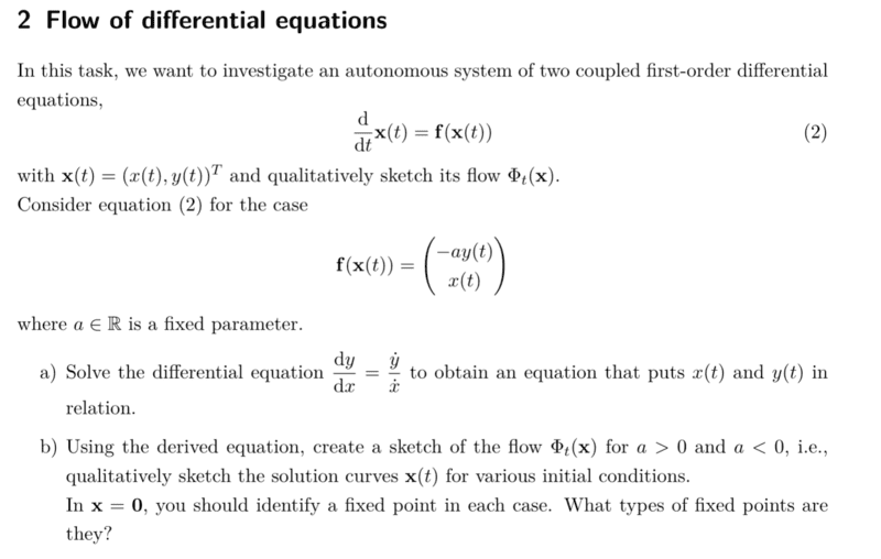
- solve the two coupled first-order differential equations ##\textbf{f}(\textbf{x}(t))## and sketch the flow ##\phi_t(\textbf{x})##
- Relevant Equations
- none
Hi,
unfortunately, I have a problem to solve the following task

The equation looks like this:
$$\left(\begin{array}{c} \frac{d}{dt} x(t) \\ \frac{d}{dt} y(t) \end{array}\right)=\left(\begin{array}{c} -a y(t) \\ x(t) \end{array}\right)$$
Since the following is true ##\frac{d}{dt} y(t)=x(t)## I substituted ##x(t)## into the first equation on the left hand side, obtaining a 2nd order differential equation, i.e. ##y''(t)=-ay(t)## to solve this differential equation I then used the Ansatz ##y(t)=e^{\lambda t}## and obtained the following solution.
$$y(t)=c_1 \ e^{i \sqrt{a}t}-c_2 \ e^{-i \sqrt{a}t}$$
I then obtain x(t) using ##\frac{d}{dt} y(t)=x(t)##
$$y(t)=i \ \sqrt{a} \ c_1 \ e^{i \sqrt{a}t}-i \ \sqrt{a} \ c_2 \ e^{-i \sqrt{a}t}$$
Unfortunately, I am now a bit unsure about task b. For the flow ##\phi_t(\textbf{x})## I would now simply draw the vector ##\textbf{f}(\textbf{x}(t))=\left(\begin{array}{c} -a y(t) \\ x(t) \end{array}\right)## with my solution from task a for ##y(t)## and ##x(t)##.
Unfortunately I have problems to draw the vector, because I don't know what the constants ##c_1## and ##c_2## are and unfortunately my solution from task a is complex, so do I have to plot only the real part or is my solution from task a wrong?
unfortunately, I have a problem to solve the following task
The equation looks like this:
$$\left(\begin{array}{c} \frac{d}{dt} x(t) \\ \frac{d}{dt} y(t) \end{array}\right)=\left(\begin{array}{c} -a y(t) \\ x(t) \end{array}\right)$$
Since the following is true ##\frac{d}{dt} y(t)=x(t)## I substituted ##x(t)## into the first equation on the left hand side, obtaining a 2nd order differential equation, i.e. ##y''(t)=-ay(t)## to solve this differential equation I then used the Ansatz ##y(t)=e^{\lambda t}## and obtained the following solution.
$$y(t)=c_1 \ e^{i \sqrt{a}t}-c_2 \ e^{-i \sqrt{a}t}$$
I then obtain x(t) using ##\frac{d}{dt} y(t)=x(t)##
$$y(t)=i \ \sqrt{a} \ c_1 \ e^{i \sqrt{a}t}-i \ \sqrt{a} \ c_2 \ e^{-i \sqrt{a}t}$$
Unfortunately, I am now a bit unsure about task b. For the flow ##\phi_t(\textbf{x})## I would now simply draw the vector ##\textbf{f}(\textbf{x}(t))=\left(\begin{array}{c} -a y(t) \\ x(t) \end{array}\right)## with my solution from task a for ##y(t)## and ##x(t)##.
Unfortunately I have problems to draw the vector, because I don't know what the constants ##c_1## and ##c_2## are and unfortunately my solution from task a is complex, so do I have to plot only the real part or is my solution from task a wrong?