Time-dependent Perturbation Theory

In summary, the conversation discusses the topic of time-dependent perturbation theory in chapter 9.12 of the book Introduction to Quantum Mechanics by David J. Griffiths. The person was confused about the first order correction ca(1)(t) = 1 while it equals a constant. They ask for clarification on how the constants (c's) are defined and mention that the author uses a process of successive approximations. The conversation also includes a discussion on the initial conditions and how they are assumed to hold for all orders of approximation. Ultimately, the conversation centers around understanding the first order approximation and its relationship to the initial conditions.
  • #1
Viona
49
12
Homework Statement
Why the first-order correction equals 1 instead of arbitrary constant?
Relevant Equations
Why the first-order correction equals 1 instead of arbitrary constant?
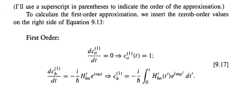
I was reading in the Book: Introduction to Quantum Mechanics by David J. Griffiths. In chapter Time-Dependent Perturbation Theory, Section 9.12. I could not understand that why he put the first order correction ca(1)(t)=1 while it equals a constant.
tdd.png
 
Physics news on Phys.org
  • #2
How are the ##c##'s defined? I ask because (1) I'm too lazy to go get my copy of Griffiths and (2) it may provide the answer to your question.
 
  • #3
vela said:
How are the ##c##'s defined? I ask because (1) I'm too lazy to go get my copy of Griffiths and (2) it may provide the answer to your question.
He used a process of successive approximations, so for this two particle system the particle starts at state ##a##, then at time t=0: ca(0)=1 and cb(0)=0. If there were no perturbation the system will stay there forever, so we can say the zeroth- order terms are: ca(t)=1 and cb(t)=0. To calculate the first order terms we plug the zeroth order terms in the equations [9.13] below:
sddd.png
 
  • #4
Viona said:
I could not understand that why he put the first order correction ca(1)(t)=1 while it equals a constant.
Recall equation [9.15], which says ##c_a(0) = 1##.
 
  • #5
TSny said:
Recall equation [9.15], which says ##c_a(0) = 1##.
In equation [9.15] ##c_a(0) = 1## this is before the perturbation (at time ##t= 0##) no transition happened yet and the particle still in the upper state ##a##. But equation [9.17] after perturbation at time t and ca(1)(t) = 1 is the first-order correction. I understand that the zeroth-order ##c_a(t) = 1## but why the first-order correction also =1?
 
  • #6
Viona said:
In equation [9.15] ##c_a(0) = 1## this is before the perturbation (at time ##t= 0##) no transition happened yet and the particle still in the upper state ##a##. But equation [9.17] after perturbation at time t and ##c_a(1)(0) = 1## is the first-order correction. I understand that the zeroth-order ##c_a(t) = 1## but why the first-order correction also =1?
How many constant functions do you know that fulfill ##c_a(0)=1##?
 
  • #7
Viona said:
In equation [9.15] ##c_a(0) = 1## this is before the perturbation (at time ##t= 0##) no transition happened yet and the particle still in the upper state ##a##. But equation [9.17] after perturbation at time t and ca(1)(t) = 1 is the first-order correction. I understand that the zeroth-order ##c_a(t) = 1## but why the first-order correction also =1?

Initially I agreed with you, but the passage in your original post defines [itex]c^{(1)}[/itex] not as the "first order correction" but the "first order approximation".

To my mind, if we speak of perturbing a system [itex]y' = f(x,y)[/itex] subjec to [itex]y(0) = 1[/itex] then the perturbed system is [itex]y' = f(x,y) + \epsilon g(x,y)[/itex] for some small parameter [itex]\epsilon[/itex]. We would then pose an expansion of the form [itex]y(x) = y_0(x) + \epsilon y_1(x) + \dots[/itex], and we would then call [itex]y_1[/itex] the first order correction. And if we don't perturb the initial condition as well then indeed [itex]y_0(0) = 1[/itex] and [itex]y_1(0) = 0[/itex].

But here the text (at least the parts you've posted) doesn't mention a small parameter, and you have described the author's method as "successive approximation" rather than "asymptotic expansion". This would be like obtaining approximate solutions to our perturbed system by the iterative process [tex]
y_{n+1}(x) = 1 + \int_0^x f(x,y_n(x)) + \epsilon g(x,y_n(x))\,dx[/tex] for which [itex]y_n(0) = 1[/itex] always holds.
 
  • #8
Viona said:
He used a process of successive approximations, so for this two particle system the particle starts at state ##a##, then at time t=0: ca(0)=1 and cb(0)=0. If there were no perturbation the system will stay there forever, so we can say the zeroth- order terms are: ca(t)=1 and cb(t)=0. T
The initial conditions at ##t = 0## are assumed to hold for all orders of approximation. So, when you solve the first-order equation ##\dot c_a(t) = 0##, you can use the initial condition ##c_a(0) = 1## to show that ##c_a(t) = 1## for all ##t \ge 0## for the first-order approximation.
 
  • #9
pasmith said:
Initially I agreed with you, but the passage in your original post defines [itex]c^{(1)}[/itex] not as the "first order correction" but the "first order approximation".

To my mind, if we speak of perturbing a system [itex]y' = f(x,y)[/itex] subjec to [itex]y(0) = 1[/itex] then the perturbed system is [itex]y' = f(x,y) + \epsilon g(x,y)[/itex] for some small parameter [itex]\epsilon[/itex]. We would then pose an expansion of the form [itex]y(x) = y_0(x) + \epsilon y_1(x) + \dots[/itex], and we would then call [itex]y_1[/itex] the first order correction. And if we don't perturb the initial condition as well then indeed [itex]y_0(0) = 1[/itex] and [itex]y_1(0) = 0[/itex].

But here the text (at least the parts you've posted) doesn't mention a small parameter, and you have described the author's method as "successive approximation" rather than "asymptotic expansion". This would be like obtaining approximate solutions to our perturbed system by the iterative process [tex]
y_{n+1}(x) = 1 + \int_0^x f(x,y_n(x)) + \epsilon g(x,y_n(x))\,dx[/tex] for which [itex]y_n(0) = 1[/itex] always holds.
He said he is going to use a process of successive approximations, I am not familiar with the "asymptotic expansion" so I can not tell if this what he did
as.png
 

FAQ: Time-dependent Perturbation Theory

What is Time-dependent Perturbation Theory?

Time-dependent Perturbation Theory is a mathematical tool used in quantum mechanics to study the behavior of a quantum system when it is subjected to an external perturbation or disturbance over time. It allows us to calculate the time evolution of a quantum system and how it responds to changes in its environment.

How is Time-dependent Perturbation Theory different from Time-independent Perturbation Theory?

Time-dependent Perturbation Theory deals with systems that are changing over time, while Time-independent Perturbation Theory is used for systems that are in a steady state or do not change with time. Time-dependent Perturbation Theory takes into account the time evolution of the system, while Time-independent Perturbation Theory only considers the perturbation at a single moment in time.

What are the applications of Time-dependent Perturbation Theory?

Time-dependent Perturbation Theory is used in many areas of quantum mechanics, such as atomic and molecular physics, solid state physics, and quantum field theory. It is also used in other fields, including chemistry, biology, and engineering, to study the behavior of complex systems under external influences.

What are the limitations of Time-dependent Perturbation Theory?

Time-dependent Perturbation Theory is limited to small perturbations and short time intervals. If the perturbation is too large or the time interval is too long, the theory may not accurately predict the behavior of the system. In addition, it is only applicable to systems that can be described by quantum mechanics and may not be suitable for classical systems.

How is Time-dependent Perturbation Theory solved?

Time-dependent Perturbation Theory is solved using mathematical techniques such as perturbation series, variational methods, and numerical methods. These methods involve expanding the time-dependent wavefunction in terms of a series of perturbations and solving for the coefficients of the series. The solutions can then be used to calculate the time evolution of the system and the probabilities of different outcomes.

Similar threads

Back
Top