Triangular cavity thermal radiation simulation

In summary, the conversation involved solving a problem related to radiation in a triangular cavity. The problem involved finding the temperature and heat flux for different surfaces with given lengths and emissivities. The person asking the question had both numerical and analytical solutions but wanted to understand the latter better. They shared their approach, based on a book by A. Bejan, and the equations they used. Another person provided a simplified version of the equations and used a code in octave (similar to Matlab) to solve them. The results were close to the expected values but not exact.
  • #1
FEAnalyst
346
147
TL;DR Summary
How to solve this problem involving radiation in a triangular cavity?
Hi,

I'm trying to solve a problem involving radiation in a triangular cavity:
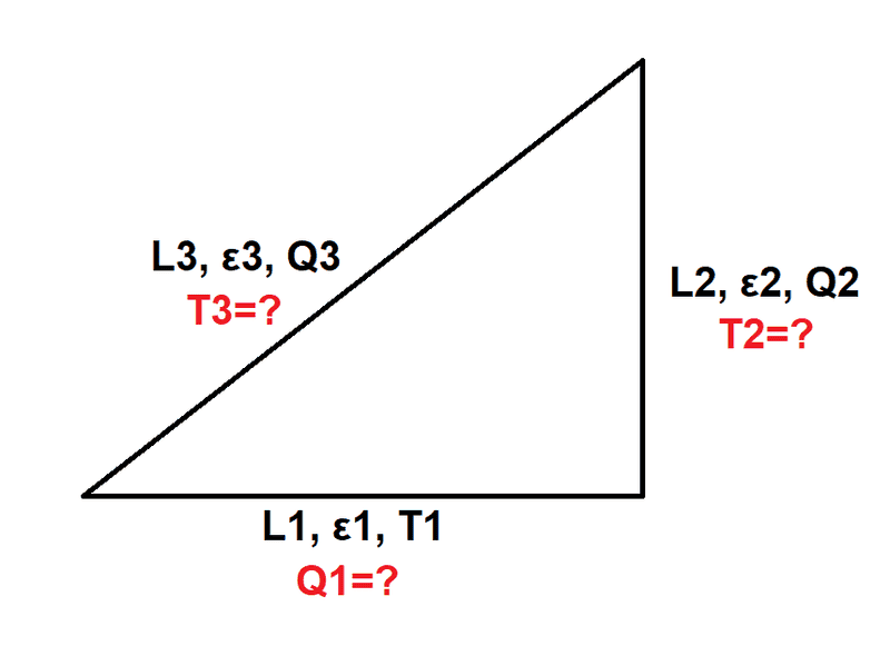
cavity.png

As you can see, lengths and emissivities of all surfaces are given. For two of them, the heat flux is known and the temperature has to be found while for the remaining surface it's the other way around.

I have the numerical and analytical solutions for this problem, but I want to know exactly how to obtain the latter. Here's my approach, based on the book by A. Bejan: $$Q_{1}=\frac{\varepsilon_{1} \cdot A_{1}}{1- \varepsilon_{1}} \cdot \left( \sigma \cdot T_{1}^{4}-J_{1} \right)$$ $$Q_{2}=\frac{\varepsilon_{2} \cdot A_{2}}{1- \varepsilon_{2}} \cdot \left( \sigma \cdot T_{2}^{4}-J_{2} \right)$$ $$Q_{3}=\frac{\varepsilon_{3} \cdot A_{3}}{1- \varepsilon_{3}} \cdot \left( \sigma \cdot T_{3}^{4}-J_{3} \right)$$ $$J_{1}=(1- \alpha_{1}) \cdot \left( (J_{2} \cdot F_{12})+(J_{3} \cdot F_{13}) \right) + \varepsilon_{1} \cdot \sigma \cdot T_{1}^{4}$$ $$J_{2}=(1- \alpha_{2}) \cdot \left( (J_{1} \cdot F_{21})+(J_{3} \cdot F_{23}) \right) + \varepsilon_{2} \cdot \sigma \cdot T_{2}^{4}$$ $$J_{3}=(1- \alpha_{3}) \cdot \left( (J_{1} \cdot F_{31})+(J_{2} \cdot F_{32}) \right) + \varepsilon_{3} \cdot \sigma \cdot T_{3}^{4}$$ where view factors are calculated from the following formulas: $$F_{12}=\frac{L_{1}+L_{2}-L_{3}}{2 \cdot L_{1}}$$ $$F_{13}=\frac{L_{1}+L_{3}-L_{2}}{2 \cdot L_{1}}$$ $$F_{31}=\frac{L_{3}+L_{1}-L_{2}}{2 \cdot L_{3}}$$ $$F_{21}=\frac{L_{2}+L_{1}-L_{3}}{2 \cdot L_{2}}$$ $$F_{23}=\frac{L_{2}+L_{3}-L_{1}}{2 \cdot L_{2}}$$ $$F_{32}=\frac{L_{3}+L_{2}-L_{1}}{2 \cdot L_{3}}$$
The problem is that the software that I use to solve this system of 6 equations for the 6 variables ##J_{1}##, ##J_{2}##, ##J_{3}##, ##Q_{1}##, ##T_{2}## and ##T_{3}## doesn't give any solution so I assume that something is wrong with my equations. Do you know where I made the mistake in the calculations? Maybe I misinterpreted the formulas from Bejan's book. They look like this: $$Q_{i}=\frac{\varepsilon_{i} A_{i}}{1- \varepsilon_{i}} \cdot \left( \sigma T_{i}^{4}-J_{i} \right)$$ $$J_{i}=(1-\alpha_{i}) \sum_{j=1}^{n} J_{j}F_{ij}+ \varepsilon_{i} \sigma T_{i}^{4}$$ for ##i=1,2,...,n## where ##n## is the number of surfaces in a cavity. $$F_{ij}=\frac{L_{i}+L_{j}-L_{k}}{2L_{i}}$$
 
Engineering news on Phys.org
  • #2
[EDIT] I've resolved a bug, in the R matrix i used -1 instead of Q2 and Q3[/EDIT]

I don't really know about radiation and so I cannot check the equations themselves. But you can just solve them as a set of 6 linear equations with 6 unknowns. First, to make things a little bit easier, define these constants:
$$
c_x = \frac{\varepsilon_x A_x}{1-\varepsilon_x}
$$
and
$$
\beta_x = 1-\alpha_x
$$
Furthermore I solve for ##T_x^4## because all temperatures enter the equation to the power four, so you don't have to bother with powers of 1/4th and all that. Just do that at the end.

Now you can just rewrite the six equations to set up this matrix equation:
$$
\begin{bmatrix}
c_1 & 0 & 0 & 1 & 0 & 0 \\
0 & c_2 & 0 & 0 & -c_2\sigma & 0 \\
0 & 0 & c_3 & 0 & 0 & -c_3\sigma \\
1 & -\beta_1 F_{12} & -\beta_1 F_{13} & 0 & 0 & 0 \\
-\beta_2 F_{21} & 1 & -\beta_2 F_{23} & 0 & -\varepsilon_2 \sigma & 0 \\
-\beta_3 F_{31} & -\beta_3 F_{32} & 1 & 0 & 0 & -\varepsilon_3 \sigma
\end{bmatrix}
\begin{bmatrix}
J_1 \\
J_2 \\
J_3 \\
Q_1 \\
T_2^4 \\
T_3^4
\end{bmatrix}
=
\begin{bmatrix}
c_1 \sigma T_1^4 \\
-Q_2 \\
-Q_3 \\
\varepsilon_1 \sigma \\
0 \\
0
\end{bmatrix}
$$

So I've used a simple bit of octave (Matlab) code to solve all this. I needed specific numbers so I just came up with a few. But you can solve above matrix analytically as well if you want.
Octave/Matlab:
L1 = 3;
L2 = 4;
L3 = 5;

eps1 = 0.3;
eps2 = 0.5;
eps3 = 0.6;

T4_1 = 200^4;
Q2 = 1500;
Q3 = 2500;

F12 = (L1 + L2 - L3)/2/L1;
F13 = (L1 + L3 - L2)/2/L1;
F31 = (L3 + L1 - L2)/2/L3;
F21 = (L2 + L1 - L3)/2/L2;
F23 = (L2 + L3 - L1)/2/L2;
F32 = (L3 + L2 - L1)/2/L3;

s = 5.670373e-8;

alfa1 = 0.8;
alfa2 = 0.7;
alfa3 = 0.1;

d = 1.2;

A1 = L1*d;
A2 = L2*d;
A3 = L3*d;

c1 = eps1*A1/(1-eps1);
c2 = eps2*A2/(1-eps2);
c3 = eps3*A3/(1-eps3);

b1 = 1-alfa1;
b2 = 1-alfa2;
b3 = 1-alfa3;

M = [
c1   0  0   1     0     0;
0   c2  0   0 -c2*s     0;
0    0 c3   0     0 -c3*s;
1 -b1*F12 -b1*F13 0  0 0;
-b2*F21 1 -b2*F23 0 -eps2*s 0;
-b3*F31 -b3*F32 1 0 0 -eps3*s
]

R = [
c1*s*T4_1;
-Q2
-Q3
eps1*s
0
0];

x = M \ R;

J1 = x(1);
J2 = x(2);
J3 = x(3);
Q1 = x(4);
T4_2 = x(5);
T4_3 = x(6);

disp(['J1 = ' num2str(J1)])
disp(['J2 = ' num2str(J2)])
disp(['J3 = ' num2str(J3)])
disp(['Q1 = ' num2str(Q1)])
disp(['T2^4 = ' num2str(T4_2) ', T2 = ' num2str(T4_2^(1/4))])
disp(['T3^4 = ' num2str(T4_3) ', T3 = ' num2str(T4_3^(1/4))])

If I run this, this is the result, for which I have no clue whether it is reasonable or not :):
Solution:
J1 = 696.1098
J2 = 2258.1934
J3 = 4091.7266
Q1 = -934.0207
T2^4 = 45335526345.2526, T2 = 461.4341
T3^4 = 77058500323.9253, T3 = 526.872
 
Last edited:
  • Like
Likes berkeman
  • #3
@Arjan82 Thank you very much. I don't have access to Matlab so I used this code in Scilab. It seems that the equations are correct from the mathematical point of view. I don't know why I wasn't able to solve them in another software.

Anyway, I substituted the input values to your code and the results are close to what I expected but not exactly. Here are the inputs: $$L_{1}=4 \ m, \ L_{2}=3 \ m, \ L_{3}=5 \ m$$ $$A_{1}=L_{1} \cdot 1, \ A_{2}=L_{2} \cdot 1, \ A_{3}=L_{3} \cdot 1$$ $$\varepsilon_{1}=\alpha_{1}=0.4, \ \varepsilon_{2}=\alpha_{2}=0.6, \ \varepsilon_{3}=\alpha_{3}=0.8$$ $$T_{1}=307 \ K, \ Q_{2}=6000 \ W, \ Q_{3}=5000 \ W$$ $$\sigma=5.67 \cdot 10^{-8} \ \frac{W}{m^{2}K}$$ And the results should be: $$Q_{1}=-11000 \ \frac{W}{m}, \ T_{2}=641 \ K, \ T_{3}=600 \ K$$ This Scilab code:

Scilab - input:
L1 = 4;
L2 = 3;
L3 = 5;
eps1 = 0.4;
eps2 = 0.6;
eps3 = 0.8;
T4_1 = 307^4;
Q2 = 6000;
Q3 = 5000;
F12 = (L1 + L2 - L3)/2/L1;
F13 = (L1 + L3 - L2)/2/L1;
F31 = (L3 + L1 - L2)/2/L3;
F21 = (L2 + L1 - L3)/2/L2;
F23 = (L2 + L3 - L1)/2/L2;
F32 = (L3 + L2 - L1)/2/L3;
s = 5.67e-8;
alfa1 = 0.4;
alfa2 = 0.6;
alfa3 = 0.8;
d = 1;
A1 = L1*d;
A2 = L2*d;
A3 = L3*d;
c1 = eps1*A1/(1-eps1);
c2 = eps2*A2/(1-eps2);
c3 = eps3*A3/(1-eps3);
b1 = 1-alfa1;
b2 = 1-alfa2;
b3 = 1-alfa3;
M = [
c1   0  0   1     0     0;
0   c2  0   0 -c2*s     0;
0    0 c3   0     0 -c3*s;
1 -b1*F12 -b1*F13 0  0 0;
-b2*F21 1 -b2*F23 0 -eps2*s 0;
-b3*F31 -b3*F32 1 0 0 -eps3*s
]
R = [
c1*s*T4_1;
-Q2
-Q3
eps1*s
0
0];
R
x = M \ R;
J1 = x(1);
J2 = x(2);
J3 = x(3);
Q1 = x(4);
T4_2 = x(5);
T4_3 = x(6);
J1
J2
J3
Q1
T4_2^(1/4)
T4_3^(1/4)

gave me the following outputs:

Scilab - output:
Q1 = -9656.9095
T4_2^(1/4) = 632.85074
T4_3^(1/4) = 589.11785

It's pretty close but there must be some mistake causing the difference. Do you know what can be wrong here? I'm specifically unsure about the areas (I assumed the depth of ##1 \ m##), absorptivities (I treated them as equal to emissivities) and formulas for view factors but other parts of the code may also be wrong.
 
  • #4
Why are you so sure these are the correct results? Where do they come from?

You can always check the results by multiplying ##M## with ##x## which should give you back the right hand side ##R##. I get exactly the same results as you and I also get back ##R## if I do the multiplication.

The only thing that could be going on numerically is that if you have a large range of values in ##M## like here, you can get into trouble with significant digits. But then again, I don't really think that this is going on.

So it then must be in the modelling.
 
  • #5
Arjan82 said:
Why are you so sure these are the correct results? Where do they come from?
Here's the source of the correct results (pages 6-7): https://www.comsol.com/model/download/646601/models.heat.cavity_radiation.pdf
They are also confirmed by simulations.

That document doesn't include the details of analytical calculations so I had to figure them out using the referenced book by Bejan. It's likely that I made some mistake but it must be rather small since the outputs are pretty close to the expected values.
 
Last edited:
  • #6
FEAnalyst said:
That document doesn't include the details of analytical calculations

It turns out it contains all information needed, from page 7:
$$
\begin{align}
Q_i &= L_i\frac{\varepsilon_i}{1-\varepsilon_i}(\sigma T_i^4 - J_i) \nonumber \\
Q_i &= L_i \sum_k F_{ik}(J_i - J_k) \nonumber \\
F_{ij} &= \frac{L_i + L_j - L_k}{2L_i} \nonumber
\end{align}
$$
Note, that no ##\alpha##'s are needed here. So, for the second equation you get
$$
Q_1 = L_1\left[F_{12}(J_1 -J_2) + F_{13}(J_1 -J_3)\right]
$$
Etc...

This then results in the next matrix equation:
$$
\begin{bmatrix}
c_1 & 0 & 0 & 1 & 0 & 0 \\
0 & c_2 & 0 & 0 & -c_2\sigma & 0 \\
0 & 0 & c_3 & 0 & 0 & -c_3\sigma \\
-L_1(F_{12} + F_{13}) & L_1 F_{12} & L_1 F_{13} & 1 & 0 & 0 \\
L_2 F_{21} & -L_2(F_{21} + F_{23}) & L_2 F_{23} & 0 & 0 & 0 \\
L_3 F_{31} & L_3 F_{32} & -L_3 (F_{31} + F_{32}) & 0 & 0 & 0
\end{bmatrix}
\begin{bmatrix}
J_1 \\
J_2 \\
J_3 \\
Q_1 \\
T_2^4 \\
T_3^4
\end{bmatrix}
=
\begin{bmatrix}
c_1 \sigma T_1^4 \\
-Q_2 \\
-Q_3 \\
0 \\
-Q_2 \\
-Q_3
\end{bmatrix}
$$

And in exactly the same way as before I now get the correct solution:
Solution:
J1 = 4628.659
J2 = 8265.0226
J3 = 7083.2044
Q1 = -11000
T2 = 641.4362
T3 = 599.6912
 
  • #7
This solution actually makes much more sense since all fluxes add up to zero now ##Q_1 + Q_2 + Q_3 = 0##. I've checked this before but it didn't work out. I just thought I just didn't understand something about this problem. As I said, I don't know too much about radiation.

So in your first post, the equations for ##J_i## don't seem to fit this model. Also, ##\alpha##'s are not important because, since the cavity is enclosed, all radiation gets absorbed eventually.
 
  • #8
@Arjan82 Thanks a lot again. So, to sum up, the system of 6 equations should look like this: $$Q_{1}= L_{1} \frac{\varepsilon_{1}}{1- \varepsilon_{1}}(\sigma T_{1}^4 - J_{1})$$ $$Q_{2}= L_{2} \frac{\varepsilon_{2}}{1- \varepsilon_{2}}(\sigma T_{2}^4 - J_{2})$$ $$Q_{3}= L_{3} \frac{\varepsilon_{3}}{1- \varepsilon_{3}}(\sigma T_{3}^4 - J_{3})$$ $$Q_{1} = L_{1} \left( F_{12} (J_{1} -J_{2}) + F_{13} (J_{1} -J_{3}) \right)$$ $$Q_{2} = L_{2} \left( F_{21} (J_{2} -J_{1}) + F_{23} (J_{2} -J_{3}) \right)$$ $$Q_{3} = L_{3} \left( F_{31} (J_{3} -J_{1}) + F_{32} (J_{3} -J_{2}) \right)$$ And the Scilab code is:
Scilab - fixed input:
L1 = 4;
L2 = 3;
L3 = 5;
eps1 = 0.4;
eps2 = 0.6;
eps3 = 0.8;
T1_4 = 307^4;
Q2 = 6000;
Q3 = 5000;
F12 = (L1 + L2 - L3)/2/L1;
F13 = (L1 + L3 - L2)/2/L1;
F31 = (L3 + L1 - L2)/2/L3;
F21 = (L2 + L1 - L3)/2/L2;
F23 = (L2 + L3 - L1)/2/L2;
F32 = (L3 + L2 - L1)/2/L3;
s = 5.67e-8;
c1 = L1*eps1/(1-eps1);
c2 = L2*eps2/(1-eps2);
c3 = L3*eps3/(1-eps3);
M = [
c1   0  0   1     0     0;
0   c2  0   0 -c2*s     0;
0    0 c3   0     0 -c3*s;
-L1*(F12+F13) L1*F12 L1*F13 1  0 0;
L2*F21 -L2*(F21+F23) L2*F23 0 0 0;
L3*F31 L3*F32 -L3*(F31+F32) 0 0 0
]
R = [
c1*s*T1_4;
-Q2
-Q3
0
-Q2
-Q3];
R
x = M \ R;
J1 = x(1);
J2 = x(2);
J3 = x(3);
Q1 = x(4);
T2_4 = x(5);
T3_4 = x(6);
J1
J2
J3
Q1
T2_4^(1/4)
T3_4^(1/4)

Now it also works in the other software in which I was trying to solve the initial, incorrect system of equations.

In fact, what confused me is this sentence from the referenced document:
Substituting this expression for the view factor into the second equation for the heat fluxes results in a linear system of six equations.
I thought that just the second equation for heat flux is needed to obtain the system of 6 equations and I was wondering how they did that so I reached for Bejan's book referenced by them and used the equations from it. Apparently, they are too general or not adjusted for this case.
 
  • #9
So now I'm curious what other software you used to solve the equations :)
 
  • #10
Arjan82 said:
So now I'm curious what other software you used to solve the equations :)
It's SMath Studio - free (but with some limitations like the limit of 3 devices per account introduced to new versions) equivalent of MathCAD. However, to solve this system of equations I had to use the Maxima plug-in for SMath. Maxima is open-source and truly free CAS software similar to Mathematica. It has its own GUI (wxMaxima) but SMath adds handling of units and a much more user-friendly display of formulas.

smath.JPG


Unfortunately, I had to suppress the units for the equation since the software reported some inconsistency of units (there can be issues with temperatures sometimes).
 
  • Like
Likes Arjan82

FAQ: Triangular cavity thermal radiation simulation

What is a triangular cavity thermal radiation simulation?

A triangular cavity thermal radiation simulation is a type of computer simulation that models the behavior of thermal radiation within a triangular-shaped cavity. It takes into account factors such as the shape and material of the cavity, as well as the temperature and emissivity of its surfaces, to predict the distribution of thermal radiation within the cavity.

What is the purpose of conducting a triangular cavity thermal radiation simulation?

The purpose of conducting a triangular cavity thermal radiation simulation is to gain a better understanding of how thermal radiation behaves in a specific scenario. This information can be used to optimize the design of thermal systems, such as heat exchangers or solar collectors, and to predict the temperature distribution within a cavity.

What are some applications of triangular cavity thermal radiation simulation?

Triangular cavity thermal radiation simulations have a wide range of applications, including in the design of solar energy systems, thermal insulation materials, and electronic devices. They are also used in the study of heat transfer and energy efficiency in buildings and industrial processes.

How is a triangular cavity thermal radiation simulation conducted?

A triangular cavity thermal radiation simulation is typically conducted using computer software, such as computational fluid dynamics (CFD) programs. The simulation involves creating a 3D model of the cavity, assigning material properties and boundary conditions, and then solving the equations that govern thermal radiation to predict its behavior within the cavity.

What are some limitations of triangular cavity thermal radiation simulations?

One limitation of triangular cavity thermal radiation simulations is that they rely on simplifying assumptions and idealized conditions, which may not accurately reflect real-world scenarios. Additionally, the accuracy of the simulation results depends on the accuracy of the input parameters and the quality of the computational methods used.

Similar threads

Replies
30
Views
4K
Replies
34
Views
5K
Replies
3
Views
1K
Replies
2
Views
2K
Replies
16
Views
1K
Replies
4
Views
2K
Replies
11
Views
677
Replies
22
Views
907
Back
Top