Understanding the probability density function

In summary, the conversation is about understanding how to interpret and create a probability density function plot from a set of data. The individual is trying to adjust the graph and data so that the mean is in the middle and the x values represent 1, 2, and 3 standard deviations from the mean. They also have questions about the meaning of certain percentages and multipliers in relation to the data. They received some guidance on plotting the data and using a known distribution to create the graph, but they also want to understand how to do it without assuming a specific distribution. The conversation ends with clarification on the meaning and origin of certain percentages and multipliers.
  • #1
tomtomtom1
160
8
Hi all

This is not a homework question but something work related which I am having difficulty understanding which I was hoping someone from the community could help me with.

I am trying to understand how to interpret & create the probability density function plot from a set of data.

For example:-
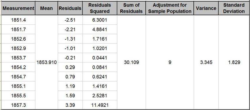
  • Below is a set of measurements of the same table which I measured 10 times.
P1.JPG


  • As you can see I have calculated the Mean, Residuals, Squared the residuals and summed up the Squared Residuals.
  • Because I can measure the table an infinite number of times (but impossible to do so) I only measured it 10 times, so 10 is my sample population and I have been told that I need to subtract 1 from the sample population which I have done so.
  • I have then calculated the variance and standard deviation.
I have then used each measurement of my table along with the mean and standard deviation and put them through the probability density function. This is what I get:-

P2.JPG


By plotting the measurements of my table (x) against the PDF (y) I get the following plot.
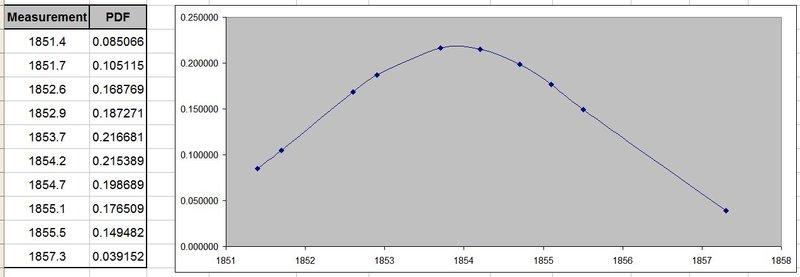
p3.JPG


I know that to find the probability of a measurement of my table to fall between 1852 - 1855 for example then I would need to integrate the P.D.F from 1855 and subtract it from the integral of the PDF to 1852.

Hopefully I have got things correct so far.

The question is how do I adjust this graph and data so that the mean is exactly in the middle and the x values are 1 2 and 3 standard deviations as shown in the example plot below:-
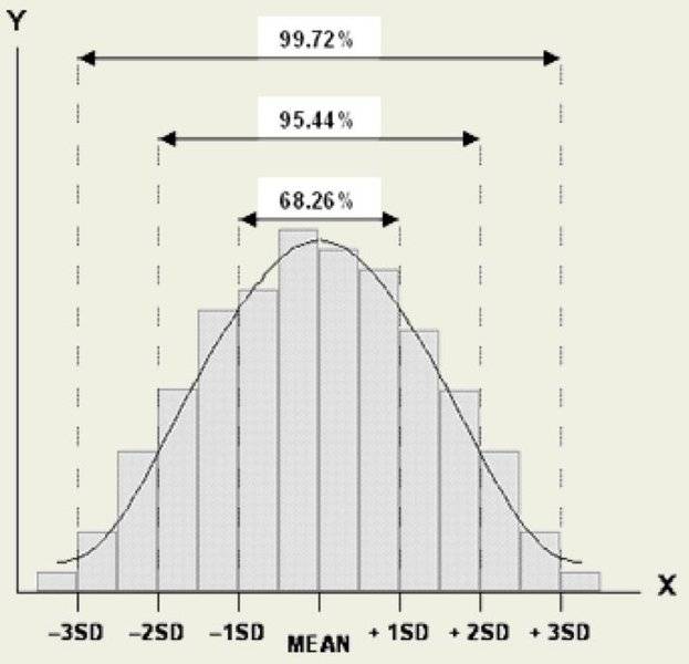
P4.JPG


I know this is a very long winded question but I could really appreciate your insight.

I have attached a note pad file that contains this data.

Many thanks.
 

Attachments

  • PDF Data.txt
    766 bytes · Views: 587
Mathematics news on Phys.org
  • #2
Is it just a plotting question?
Based on the mean and standard deviation estimated from your measurements, you can make a new table where you use (mean), (mean +- 1 standard deviation), (mean +-2 standard devations) and so on as points.
 
  • #3
If you have a good reason to assume a known distribution of the random variable that you are sampling, then you can just plot that equation using the parameter estimates from the sample. In this case, if you know that the data is from a normal distribution, then you have an equation that you can plot.

If you want to base a graph only on the data without assuming that the data came from a particular distribution, then you can do it this way: First plot points of the sample cumulative distribution. Then fit a smooth curve through the points making sure that it starts at 0 at the bottom and ends at 1 at the top. Finally, plot the slopes of the CDF curve to get a PDF.
 
  • #4
mfb said:
Is it just a plotting question?
Based on the mean and standard deviation estimated from your measurements, you can make a new table where you use (mean), (mean +- 1 standard deviation), (mean +-2 standard devations) and so on as points.

Thanks I managed to re-arrange the data into a new table.
 
  • #5
mfb said:
Is it just a plotting question?
Based on the mean and standard deviation estimated from your measurements, you can make a new table where you use (mean), (mean +- 1 standard deviation), (mean +-2 standard devations) and so on as points.

mfb

Thank your response, I was hoping you could explain two additional queries I am having trouble with.The first is this, my Mean is 1853.910 and SD is 1.829. I have integrated the probability density function from :-
  • -1SD to +1SD (1852.081 - 1855.739) and I get a value of 68.269%.
  • -2SD to +2SD (1850.252 - 1857.568) and I get a value of 95.44997%
  • -3SD to +3SD (1848.423 - 1859.397) and I get a value of 99.73707%

My question is what does 68.269%, 95.44997%, 99.73707% actually mean?

What does it mean to say that between +/- 1 SD it is 68.269%.

I think (but hoping you can confirm) that what 68.269% means is that if I randomly pick a measurement from my data set then there is a 68.269% chance that the measurement will fall within +/- 1SD.

Or can I say that for the data set to be considered a normal distribution then 68.269% of the measurements must fall within +/- 1SD.

Have I got this completely incorrect and misinterpreted? how would you explain what 68.269% means?The second question is what people call multipliers, for example:-
  • 95% = 1.96 * Standard Deviation
  • 99.7% = 2.935 * Standard Deviation
Where does 1.96 and 2.935 (which are referred to as multipliers) come from? and why does multiplying 1.96 by the standard deviation result in 95%? I thought the percentage values come from integrating the probability density function.

Can help explain or clarify?

Thanks
 
  • #6
tomtomtom1 said:
I think (but hoping you can confirm) that what 68.269% means is that if I randomly pick a measurement from my data set then there is a 68.269% chance that the measurement will fall within +/- 1SD.
If you randomly pick a measurement from a distribution that follows a Gaussian distribution, you get this probability. If you re-measure the length again, you get this probability that the value will be within +-1 SD.
If you randomly pick from your small set of measurements, the probability will be something else.
tomtomtom1 said:
Where does 1.96 and 2.935 (which are referred to as multipliers) come from?
They are chosen to get 95% or 99.7% as integral, respectively. It doesn't make sense to write an equal sign there. They are just more entries to the table of "x% of the measurements will be within y SD of the mean" in the same way as you made three already.
 
  • #7
mfb said:
If you randomly pick a measurement from a distribution that follows a Gaussian distribution, you get this probability. If you re-measure the length again, you get this probability that the value will be within +-1 SD.
If you randomly pick from your small set of measurements, the probability will be something else.They are chosen to get 95% or 99.7% as integral, respectively. It doesn't make sense to write an equal sign there. They are just more entries to the table of "x% of the measurements will be within y SD of the mean" in the same way as you made three already.
Hi mfbAgain thank you for your insight.You the following:-If you re-measure the length again, you get this probability that the value will be within +-1 SD - This makes a lot of sense to me.However your comment about:-If you randomly pick from your small set of measurements, the probability will be something else.Correct me if I am wrong but I have 10 measurements, if I randomly pick a measurement from this small data set then the probability of picking any of the measurements is equally the same 1/10 or 10%. - is this what you were referring to when you said "the probability will be something else"?If I randomly pick a measurement from this data set (where each measurement is equally likely to be picked i.e. 10%) then is it correct to say the probability of the measurement being picked has a 68.269% chance of being between +/- 1SD?Your thoughts?
 
  • #8
tomtomtom1 said:
Correct me if I am wrong but I have 10 measurements, if I randomly pick a measurement from this small data set then the probability of picking any of the measurements is equally the same 1/10 or 10%. - is this what you were referring to when you said "the probability will be something else"?
Right. You have some value of measurements within 1 standard deviation - but certainly not 6.8 measurements because that doesn't make sense.
tomtomtom1 said:
If I randomly pick a measurement from this data set (where each measurement is equally likely to be picked i.e. 10%) then is it correct to say the probability of the measurement being picked has a 68.269% chance of being between +/- 1SD?
No.

Think of rolling a die once: Before you roll you know you have a 1/6 chance to roll a 6. Afterwards you either rolled it (100% of your rolls were 6) or you did not (0% were 6), but there is no way 16.7% of your 1 rolls were 6.
 

FAQ: Understanding the probability density function

What is a probability density function (PDF)?

A probability density function (PDF) is a mathematical function that describes the probability distribution of a continuous random variable. It is used to calculate the likelihood of a continuous variable falling within a certain range of values.

How is a PDF different from a probability mass function (PMF)?

A probability mass function (PMF) is used for discrete random variables, while a probability density function (PDF) is used for continuous random variables. A PMF assigns probabilities to specific values, whereas a PDF assigns probabilities to ranges of values.

What is the relationship between a PDF and a cumulative distribution function (CDF)?

The cumulative distribution function (CDF) is the integral of the probability density function (PDF) and gives the probability of a random variable being less than or equal to a specific value. In other words, the CDF is the area under the PDF curve up to a certain point.

What is the importance of understanding the PDF in statistical analysis?

The PDF allows us to determine the likelihood of obtaining certain values for a continuous random variable. This is important in statistical analysis because it helps us understand and make predictions about real-world phenomena, such as stock prices, weather patterns, and biological processes.

How is the PDF used in practical applications?

The PDF is used in a variety of practical applications, such as risk analysis, quality control, and data modeling. It is also used in machine learning and data science to build predictive models and make data-driven decisions. Additionally, the PDF is used in fields like physics, engineering, and economics to analyze and interpret experimental data.

Back
Top