Variance of 'concatenated' distributions

[query_ious]

The below is motivated by a problem I'm observing in my experimental data

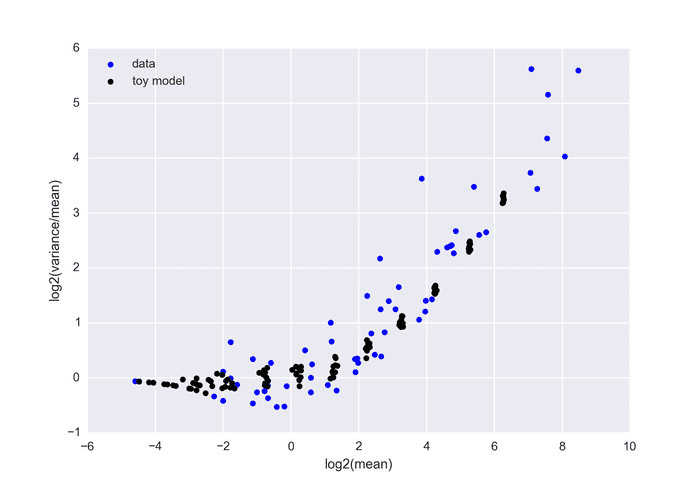
I have m boxes, where each box is supposed to contain k molecules of mRNA. The measurement process includes labeling all the molecules with a box-specific tag, mixing them, amplifying them to detectable levels and deconvoluting based on tags. As tag-labeling is a lossy process with estimated efficiency of 5-10% and as we are essentially counting successes a binomial model with n=k and 0.05<p<0.1 sounds fitting. Graphing the variance/mean vs. mean shows that it doesn't fit to the straight line expected from a binomial with constant p. If we assume that p is variable, however, things work out well. (see bottom for data)

The intuition is that we are 'concatenating' distributions - as an example assume that m/2 boxes are sampled with p=0.05 and m/2 boxes with p=0.1. Then the distribution of all m boxes would be an 'overlap' of 2 binomials each with the same n but different p. Intuitively I would expect the mean to be bound between the mean of the two distributions (as the mean is a point found between the two other points) while I would expect the variance to be larger than either of the two variances (as variance is correlated with the width of the distribution and the 'overlapping' width is by definition longer than each of its components). Simulations support my argument but I don't know how to go about formalizing it and I don't know how to use this to assist is modeling the data. (Esp - how to use this to estimate the variability in tagging efficiency).

What do you say?

The below graph shows real data (each point is generated from 24 boxes with equal k) versus the toy model suggested above (100 boxes with p=0.05 and 100 boxes with p=0.1 for different n).

[Edited for clarity + typos]

 

[mfb]

I don't see the image. Just a blank space.
Edit: Looks like some decoding problem. The image exists, but it does not get displayed correctly here. Downloading and opening it locally works.
How did you get the individual data points? Each one is one experiment with m boxes? How do they differ from each other?

Could p depend on m? That would allow to make better predictions.

For the simplified model with m/2 at p=0.05 and m/2 at p=0.10, variance should be 1/2 Var(k,p=0.05) + 1/2 Var(k,p=0.10) + (k*0.025)^2 where the last term is the deviation between mean of the total distribution (k*0.075) and mean of the individual sample distributions (k*0.05 and k*0.10 respectively).
Making more complex models is possible in the same way, but you quickly end up fitting curves to get the best model.

 

[query_ious]

I don't see the image. Just a blank space.

I see it on my screen... not sure how to fix this.

How did you get the individual data points

The setup is a bit detailed but basically this is one big experiment where a mix of ~100 RNA types is pipetted into 24 boxes such that each box gets an equal amount of mix. Each box is labeled separately and then all boxes are pooled into one big box, amplified and separated algorithmically. Each data point in the graph is generated from a 24-member list consisting of the number of estimated molecules for a certain RNA type in all 24 boxes.

Could p depend on m?

I don't expect it to but it might vary between experimental batches. I tested this and didn't see much of a difference.

For the simplified model with m/2 at p=0.05 and m/2 at p=0.10, variance should be 1/2 Var(k,p=0.05) + 1/2 Var(k,p=0.10) + (k*0.025)^2

Would you mind sharing the derivation? I'm a bit lost...

 

[mfb]

Are the "amplification process" and the detection afterwards exact? If you start with n marked RNA sequences, you will always measure that number n?

The leftmost numbers would correspond to a mean of <1/16, or just one labeled RNA sequence from a single box out of 24? Then they should have a more discrete spacing, and the data samples should not have a well-defined variance.
And what about the data point at (4,3.6)? A mean of 16, a variance of ~200? Would be interesting to see the actual distribution for those outliers.

Would you mind sharing the derivation? I'm a bit lost...

In general, if you add two distributions with known means µ₁ and µ₂ and variances V₁ and V₂, and if a fraction p comes from distribution 1 and (1-p) from distribution 2, the new mean is
$$\mu = p\mu_1 + (1-p) \mu_2$$
And the variance is
$$V = p(V_1+(\mu-\mu_1)^2) + (1-p) (V_2+(\mu-\mu_2)^2)$$
The latter formula is very similar to the parallel axis theorem in mechanics, as you are interested in the second moment in both cases.

 

[Stephen Tashi]

I have m boxes, where each box is supposed to contain k molecules of mRNA. The measurement process includes labeling all the molecules with a box-specific tag, mixing them, amplifying them to detectable levels and deconvoluting based on tags.

What does it mean to "deconvolute based on tags"?

I don't understand what you are graphing. The graph apparently shows the mean (of something) versus its variance. What is the random variable being sampled?

What makes the data points different? Are they from batches of repetitions of the above process? Or does each data point represent the sample mean and variance of a count of molecules with a given "label" taken over repetitions of the above process?