When should you use more mesh elements in the finite element method?

In summary: I'm still waiting for the statue of liberty...In summary, the conversation discusses the use of simple rectangular isoparametric elements for generating complex shapes and the high accuracy of results obtained using this method. However, it is mentioned that for more complicated shapes, multiple elements and higher order basis functions are needed to reduce numerical errors. The relationship between domain discretization and solution accuracy is also highlighted.
  • #1
mdn
49
0
TL;DR Summary
why to use more mesh elements in finite element method?
the simple rectangular isoparametric element (curved edges element) can be used to generate many complex shapes like..
square to circle
square to triangle
two square elements to annular.
and the results i calculated in python code (2D case) are very accurate, then i confused why to use complex mesh generator software etc.
for example, i calculated electric field distribution complex shape waveguide using single rectangular Lagrange element of order 4 ( it has 25 interior points). here i didn't used any mesh generator software
1661829906976.png
1661830377980.png
 
Physics news on Phys.org
  • #3
jedishrfu said:
Smaller element size improves accuracy of FEA
OfCourse this is correct. wouldn't it is possible to increase the accuracy of solution by increasing order of element (order will increase number of nodes inside the element) instead of repeating elements? i observed that 5 to 6 nodes are sufficient to gives accurate solution even for hyperbolic PDE (sine curve). as mentioned in OP even single rectangular element cover complex shape just by increasing order of element. that's why I asked question why to use large elements. no doubt for complex 3D shapes, it required meshing, but to study fundamental laws using differential equation, cross section of given material is sufficient to study it.
 
  • #4
Isn't there a risk though that your simplification will fail? Perhaps folks try it both ways and when they see the simpler mesh works they go with it otherwise they stick with more elements.
 
  • #5
suppose i have star domain as show in figure, will it required mesh generation software like gmsh etc? i will say no, this star shape can be covered (100% without discretization error) using single isoparametric rectangular element of order 2 just by displacing boundary nodes inside.
1661844544399.png
 
  • #6
mdn said:
this star shape can be covered (100% without discretization error) using single isoparametric rectangular element of order 2 just by displacing boundary nodes inside.
Try a star where one of the angles is 0.1 degrees. And the star has a round hole in the middle. And it is 3D and being held by the statue of liberty. You will have a hard time generalizing this to a lot of different shapes.

But for simple shapes, you can indeed increase the order of the basis function to 100 or so and work with a single element. That is basically spectral element methods. Convergence of the error with degrees of freedom is much faster when you increase the polynomial degree, compared to increasing the number of elements. However, your solution needs to be differentiable up to the order of the polynomial. Many practical problems are not infinitely differentiable. Shock waves for example are discontinuous and not even differentiable once in the neighborhood of the shock. This is why aerodynamics codes try to locate the position of the shock wave, and they switch to lower order schemes or use some other special tricks in the neighborhood of the shock. Or you could use discontinuous Galerkin methods, where the solution is allowed to be discontinuous from one element to the next. There are many different tools available for many different problems.
 
  • #7
bigfooted said:
Try a star where one of the angles is 0.1 degrees. And the star has a round hole in the middle
1662737232297.png
1662737910558.png

the middle is a second order rectangular element (blue dots, 9 nodes) , just displacing nodes in the direction of arrow we can generated circle of any radius. for making star, four elements of order 1 are used (4 nodes for each element). we can make any angle no matter because it is made by using Jacobin transformation with the help of Lagrange interpolation basis functions. here is no need to use any mesh generation software, just coordinates of vertices are needed to generate complex shapes. as you commented out "your solution needs to be differentiable up to the order of the polynomial" but there is no relation between domain discretization and actual solution obtained. i mean degree of polynomial used for obtaining solution may be different than the domain discretization.
 

Attachments

  • 1662736874140.png
    1662736874140.png
    6 KB · Views: 116
  • #8
I'm still waiting for the statue of liberty...
 
  • #9
mdn said:
the middle is a second order rectangular element (blue dots, 9 nodes) , just displacing nodes in the direction of arrow we can generated circle of any radius. for making star, four elements of order 1 are used (4 nodes for each element).
So it is not possible anymore to do this with a single element... I do not think you understood what I was trying to say: Your method is perfectly fine for simple geometries, but you need to use more elements to capture more complicated shapes, exactly like what you did. And these elements need to have certain geometric properties or the solution will have very high numerical errors.
mdn said:
we can make any angle no matter
No, you cannot. The solution on the domain is affected by the angle that you choose. If the angle becomes smaller, your error will increase. The usual discretization errors that are mentioned in the textbooks are only for perfect squares and triangles.
mdn said:
as you commented out "your solution needs to be differentiable up to the order of the polynomial" but there is no relation between domain discretization and actual solution obtained. i mean degree of polynomial used for obtaining solution may be different than the domain discretization.
But there is a relationship between domain discretization and the solution. Your discretization determines the solution. And the solution is determined by the number of degrees of freedom that you introduce, which is a function of the number of finite elements and the polynomial order of the elements. So: yes, the degree of the basis functions can be different per finite element. But you cannot in general choose the order of the basis functions independently from the finite element discretization.
For instance the sides of the circle need to be discretized using finite elements with at least a second order basis function to capture the geometry exactly, or you introduce an additional discretization error.

There is a nice book from Sherwin and Karniadakis, hp/spectral element methods. It discusses many of these issues.
 
  • #10
thanks for sharing "Sherwin and Karniadakis, hp/spectral element book". i was completely unaware of this element. the co-incident is that, i made complete solver without any mesh software in python which is resemble this concept. of course, "statue of liberty" is also possible! but i have to take help of Blender (modeling software, it is also made in python) for generation of node coordinates. one question i would like to ask, as you mentioned in post "If the angle becomes smaller, your error will increase". but, i just displacing nodes to make small angle in element and which is completely in accordance (obeying geometry rules) with the geometry, then why should be there error? i am not discretizing any thing. for example, i have solved Laplace equation with Dirichlet and Neumann boundary condition,
1662809641608.png
1662809892205.png
the domain and solution are shown in above figure. does it has error because of due to small angles?
i am giving snippet of codes to show how i put geometrical data and processed in solver. it is my own code except linear algebra pack.

import math
import mesh
import solver
import time
import numpy as np
from scipy.linalg import eigh
#if f and rho are time dependent then you have to pass time and store all element matrices k,f according to time. M is not time dependent
## setting functional
p=2#order of approximation. (p+1)*(p+1)=nodes, here you can increase any order basis function to compute the solution.
# relation between gauss points and degree of polynomial is: p=2n−1 where p=degree of polynomial and n=gauss points. therefore=(p-1)/2(observation: put same p=n)
solver.GP=p+1 #warning increase the gauss points according to polynomial degree otherwise, solution fluctuate
solver.F=f"0"# you can use any f(x,y) here, it is multiped with shape function in solver.
solver.RHO=f"1.0"
solver.setMassTime(massMatrix=False,time=False)# if you want to mass matrix set this true
# solver.FUNCTIONAL=f"delfx('{shape}')*delfx('{shape[j]}')+delfy('{shape}')*delfy('{shape[j]}')"
# poissons weak form is int(dNi/dx *dNj/dx + dNi/dy* dNj/dy)dxdy=int(fNi) dxdy+ int(qNi)dl
#importing mesh data
totalElements,totalNodes,npe,cords,lg,dirich,neum,robin=mesh.data('laplace_dirich.txt')
# right hand side functions f and rho are set in solver getElementMatrices()
solver.setFunctional(f"delfx($i)*delfx($j)+delfy($i)*delfy($j)",p)#$i and $j are shape functions
# if you want to use 9 element node and don't want to make higher order then use
# transEq=sh.getTransEq(cords,p)
# npe=nodes per element.
#elementsCords[elNo][localNo]=(x,y)
original_order=int(math.sqrt(npe)-1) # original nodes per element
elementsCords, npe=solver.getHigherNodes(cords,p,original_order)#[[(),(),()],[(),(),()]]
stiffMatrices,massMatrices,loads=solver.getElementMatrices(elementsCords,p)# each element cordinates, order
load=solver.setNeumannBC(elementsCords,loads,neum,p)
# stiffMatrices=solver.setRobinBC(elementsCords,stiffMatrices,robin,p)
globalNumbers,totalNodes=solver.getGlobalNumbers(elementsCords)
#you can give condition here whether you want mass matrix or not...
globalStiff,globalMass,globalLoad=solver.assemble(stiffMatrices,massMatrices,load,globalNumbers,totalNodes,p)
GK,GM,GL=solver.setDirichletBC(elementsCords,globalStiff,globalMass,globalLoad,globalNumbers,dirich,p)
##############Solving eigenvalue problem separation of variable method#############
############## Mx=lambda*Kx
# eigvals, eigvecs = eigh(GK, GM)
# cutoffWavenumbers=np.array([math.sqrt(i) for i in eigvals])
# print(cutoffWavenumbers)
# print(cutoffWavenumbers*((3*10**8)/(2*np.pi))*100)
###################################################################################
###########################solving Eliptical problem, KU=F#######################################
U=np.linalg.solve(GK,GL)
print(np.array(U).reshape((p+1),(p+1)))
####################Generating intermediate solution.
division=10
# Z,XY=solver.approximateSolution(U,elementsCords,globalNumbers,p,division)# value of division must be as like order p, and it must greater than p
Z,XY=solver.approximateSolution(U,elementsCords,globalNumbers,p,division)# value of division must be as like order p, and it must greater than p
# time to plot
x=[x for x,y in XY]
y=[y for x,y in XY]
import matplotlib.pyplot as plt
fig=plt.figure()
ax=fig.add_subplot(1,2,1,projection='3d')
# ax.scatter(x,y,Z)# all one dimensional array
ax2=fig.add_subplot(1,2,2)
ax2.scatter(x,y,color="black",s=3)
x=np.array(x).reshape(division,division)
y=np.array(y).reshape(division,division)
Z=np.array(Z).reshape(division,division)
# ax.contourf(x,y,Z)
ax.plot_surface(x,y,Z)
# ax.plot_wireframe(x,y,Z)
plt.show()
#------------------Geometrical data:

#sovled and checked...
#total element, total nodes,nodes per element
$te,1
$tn,4
$npe,4
#elementNum,localNo,x,y nodes coordinates..
$cordStart
1,1,-0.9999999776482582,-0.9999999776482582
1,2,0.980785209685564,0.19509041449055076
1,3,0.19509023986756802,0.9807853028178215
1,4,2.4243127554655075,1.9495416432619095
$cordEnd
#elementNo,localNo,globalNo: numbering # no need to give local global numbering, solver will automatically detect near by elements and gives numbering.
#max of global number is total nodes
$lgStart
$lgEnd
#elementNo,edgeNo,value
$dirichStart
1,1,0
1,3,200*x
1,4,0
1,2,200*y
$dirichEnd
#elementNo,edgeNo, value, you can wirte value as f(x,y) without quoat
$neumStart
1,3,0
1,1,0
$neumEnd
$robinStart
$robinEnd
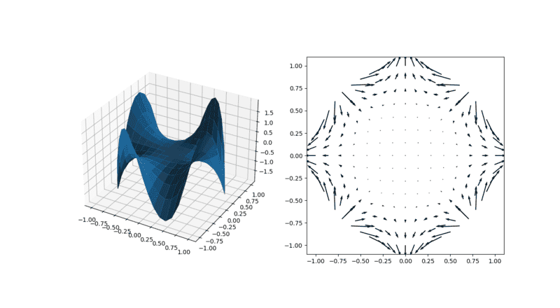
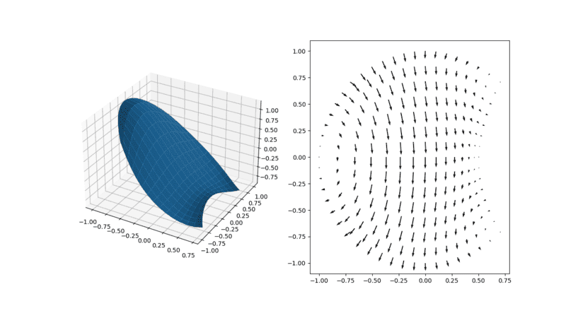
 

Attachments

  • 1662809771006.png
    1662809771006.png
    23.2 KB · Views: 129

FAQ: When should you use more mesh elements in the finite element method?

When should I use more mesh elements in the finite element method?

The number of mesh elements used in the finite element method depends on the complexity of the problem being solved. Generally, using more mesh elements can provide more accurate results, but it also increases computational time and resources. Therefore, it is important to strike a balance between accuracy and efficiency when deciding on the number of mesh elements to use.

How do I determine the optimal number of mesh elements to use?

The optimal number of mesh elements can be determined through a process called mesh refinement. This involves gradually increasing the number of elements and analyzing the results to see if there is a significant improvement in accuracy. The process should be repeated until the desired level of accuracy is achieved without a significant increase in computational time and resources.

Can using too few mesh elements affect the accuracy of my results?

Yes, using too few mesh elements can lead to inaccurate results. This is because the finite element method relies on dividing the problem domain into smaller elements to approximate the solution. If the elements are too large, the approximation will not be as accurate. Therefore, it is important to use an appropriate number of mesh elements to ensure accurate results.

Are there any specific guidelines for determining the number of mesh elements to use?

There are no specific guidelines for determining the number of mesh elements to use, as it depends on the specific problem being solved. However, some general recommendations suggest using at least 10 elements per wavelength for acoustic problems and at least 5 elements per wavelength for structural problems. It is also important to consider the aspect ratio of the elements, with a recommended maximum of 5 for accuracy.

Can I use too many mesh elements in the finite element method?

Using too many mesh elements can lead to unnecessary computational time and resources, without significant improvement in accuracy. It is important to balance the number of elements with the desired level of accuracy and efficiency. Additionally, using too many elements can also lead to numerical instability and convergence issues, so it is important to carefully consider the number of elements used in the finite element method.

Back
Top