Adding noise and solving stochastic ODEs in Python

In summary: I'm sorry if I'm being too dense. In summary, you are trying to introduce noise to the ITMblood in order to make the system more realistic. This will cause the system to flatten out as ITMblood→ITMmax and also flatten out asymptotically. You also mention that if the concentration of ITMs becomes critical, you will see a "collapse." However, I don't understand what the purpose of the noise is. Can you elaborate?
  • #1
vabsie
7
0
TL;DR Summary
I have 14 coupled ordinary differential equations. I am trying to increase the concentration of one of the ODEs by adding a sinusoidal equation that is at the same time "noisy". This noise I introduce follows a gaussian distribution with mean 0 and sigma that I vary in several experiments. I have not tried calculating for an analytical solution (not sure if even possible) but only used Python to solve the system. I don't know if I am doing it right. Any help is appreciated.
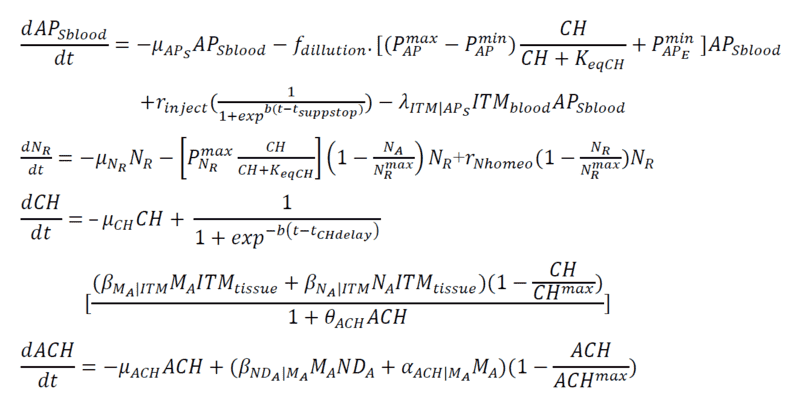
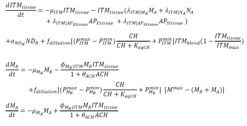
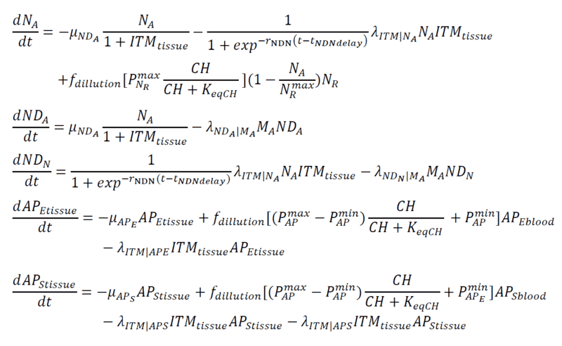
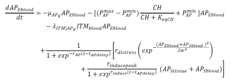
The Coupled ODE Model
Below are my coupled differential equations, where the only variable I try to meddle with is the ITMblood. The motivation here is if I try to increase ITMblood (in the next section I will show how I do it), at some concentration of ITMblood (most likely a very huge one) , the system below "collapses." That is, some of the concentrations just flattens out.

1622775454078.png

1622775479004.png

1622775533539.png

1622775563254.png

1622775606775.png

Introducing Noise to ITMblood
This is just a naive method that I am doing. So I just add a "source" of this ITMblood that follows a sinusoidal function which plateaus at rITMaddpeak and somehow starts "late" controlled by tITMadd. Then I add "noise" that simply follows a gaussian distribution with mu = 0 and sigma that I vary as part of my experiments.
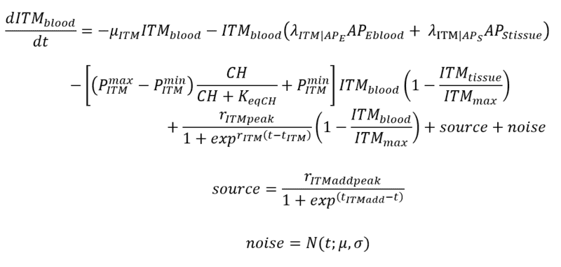
1622781855080.png


Python Library Used to Solve the Equations
scipy.integrate.odeint

note: I have tried an existing library (sdeint) specifically designed for SDEs but for some reason, the solver just can't handle the system/blows up, even when I have not added noise yet (used this as sanity check).

Am I doing this right? Does this method of introducing noise make sense? Thank you very much! I can upload my notebooks if necessary.
 

Attachments

  • 1622781639624.png
    1622781639624.png
    12.8 KB · Views: 179
  • 1622781719003.png
    1622781719003.png
    13.3 KB · Views: 188
Last edited:
Technology news on Phys.org
  • #2
Holy equation, batman! That's a lot of equations to process :oldbiggrin:

If you don't mind, I'm going to arbitrarily cut out some of your variables and make a toy model that will be easier for myself and other folks to analyze. If I end up cutting out something that's extremely relevant, please speak up.

How about a two-equation model: $$\frac{dITM_{blood}}{dt} = -\mu_{ITM} dITM_{blood} - \lambda_{ITM | AP_E} AP_{Eblood} ITM_{blood} + \frac{r_{ITMpeak}}{1+\exp[r_{ITM}(t-t_{ITM})]}\left(1 - \frac{ITM_{blood}}{ITM_{max}} \right)$$ $$\frac{dAP_{Eblood}}{dt} = -\mu_{AP_E} AP_{Eblood} - \lambda_{ITM|AP_E} ITM_{blood} AP_{Eblood}$$

What I see here is that ##ITM_{blood}## will decay if there is no source function, and that ##ITM_{blood}## has some funky time-dependent behavior that asymptotic flattens out as ##ITM_{blood} \rightarrow ITM_{max}## and also flattens out asymptotically as ##r_{ITM}t \rightarrow \infty##. If you want to observe this behavior, it seems all you need is a constant source term:
$$\frac{dITM_{blood}}{dt} = -\mu_{ITM} dITM_{blood} - \lambda_{ITM | AP_E} AP_{Eblood} ITM_{blood} + \frac{r_{ITMpeak}}{1+\exp[r_{ITM}(t-t_{ITM})]}\left(1 - \frac{ITM_{blood}}{ITM_{max}} \right) + S$$ where ##S = \mu_{ITM} ITM_{max} ##. That constant source term will cause ##ITM_{blood}## to reach equilibrium at ##ITM_{max}## where you will see flattening of the funky time-dependence. I'm not sure what you hope to accomplish with the inverse exponential source you added (also, why did you call that a sinusoidal term? that part was very confusing to me and I think it's just a matter of context). It's also not clear to me what the noise term would do for you. Can you elaborate?
 
  • #3
Twigg said:
If you don't mind, I'm going to arbitrarily cut out some of your variables and make a toy model that will be easier for myself and other folks to analyze. If I end up cutting out something that's extremely relevant, please speak up.
Go ahead! I did not want to miss out on the details, which could be important. That huge system is actually a model of the immune system. :oldbiggrin: But you're right! Trimming it down to a toy model won't hurt.
Twigg said:
What I see here is that ITMblood will decay if there is no source function
You are absolutely right! To make it comprehensible, ITM here means Inflammation Triggering Moieties or the bad things that make your immune system fire up.
Twigg said:
ITMblood has some funky time-dependent behavior that asymptotic flattens out as ITMblood→ITMmax and also flattens out asymptotically as
Yes! The sigmoidal function has an initial peak controlled by ##r_{ITMpeak}##. If the concentration of ##ITM_{blood}## closes into ##ITM_{max}##, it just stops adding up. So the following term controls the slow build up of ITMs. :woot:

$$1-\frac{ITM_{blood}}{ITM_{max}}$$

It basically means the system can only handle this much maximum concentration of ITMs.
Twigg said:
If you want to observe this behavior, it seems all you need is a constant source term:
I wanted to add a source of ITMs (as this original equation/profile for ##ITM_{blood}## eventually decays). Let's just say, some medical complications happen and suddenly we have another source of those bad things (ITMs). BUT the catch is, I wanted to make it noisy to mimic a real system (as opposed to a deterministic one).

Twigg said:
why did you call that a sinusoidal term? that part was very confusing to me
My bad! This was a typo. Let me edit it in my original post. I was referring to "sigmoidal" :nb).This is how I want to add the source term of ITMs so it won't increase linearly, and instead stop increasing at a maximum value. I hope that's clear?

So why I am adding noise? To mimic a real system! And hopefully, if the concentration of ITMs becomes critical to the system, I will see a "collapse" (I imagine this as some concentrations not going back to normal values). The noise I can "study" using early warning signals for critical transitions.

Thank you very much! I still don't know how to add the noise. My solver is sometimes throwing off errors. :frown:o_O And it is not helping because I want to do as many experiments as possible (ie varying the noise that I add).

PS
Bummer, I can't edit the original post anymore. Sinusoidal was supposed to be sigmoidal. Sorry for the confusion!
 
Last edited:
  • #4
I think I see what you mean now. Sorry if I was just saying things that were obvious! Just wanted to make sure I was reading things correctly.

Unfortunately, we would need more information to tell you why your solver (I take it this is the SDE solver?) is throwing errors, and given the size of your model we probably wouldn't be able to find the issue in our spare time. All I can really offer you on this front is I encourage you to follow best coding practices, and make sure to thoroughly unit test your function that spits out the time derivatives. If you can reproduce the SDE errors with a toy model, then we might be able to help!

If the SDE solver continues to be a problem, you could always fall back on the ODE solver and generate white noise from a normal distribution to add into your derivatives function. If you do this process many times and do good statistical inference, you should be able to learn just as much, at the expense of computational resources / time. This might actually be the less treacherous approach if you expect some kind of phase transition / bifurcation / etc.
 
  • #5
Twigg said:
If the SDE solver continues to be a problem, you could always fall back on the ODE solver and generate white noise from a normal distribution to add into your derivatives function. If you do this process many times and do good statistical inference, you should be able to learn just as much, at the expense of computational resources / time. This might actually be the less treacherous approach if you expect some kind of phase transition / bifurcation / etc.
Thank you very much! This is the approach that I am doing at the moment. I am not using the SDE solver as even with a vanilla implementation (setting noise to 0, for sanity check), it is still spewing out errors, probably because of the complexity/size of my system. I even tried doing the manual approach (Euler-Maruyama), meaning I did not use a solver but coded from scratch. But it took forever to run. Yikes.

So I am using my ODE solver for this. Sometimes, it gives me ok results, sometimes, it just gives me errors. :eek:

I guess I just have to catch the best ones!

Thank you very much for your time!
 
  • #6
vabsie said:
Sometimes, it gives me ok results, sometimes, it just gives me errors.
Does the ODE solver still spit out errors when you set the noise to 0? And does it consistently spit out errors or does it only do it for certain initial conditions? If it happens randomly with no noise and identical initial conditions, something is very wack with the derivatives function.

vabsie said:
I even tried doing the manual approach (Euler-Maruyama), meaning I did not use a solver but coded from scratch. But it took forever to run. Yikes.
yeaaah I would definitely stick to scipy
 
  • #7
Twigg said:
Does the ODE solver still spit out errors when you set the noise to 0? And does it consistently spit out errors or does it only do it for certain initial conditions? If it happens randomly with no noise and identical initial conditions, something is very wack with the derivatives function.
The ODE solver is SUPER A-OK when noise is 0. The problem happens when I add noise :H Sometimes, it gives out errors, sometimes it's ok.

Especially in one of my experiments where I add ITMs for a period of 3 hours ONLY (for example). So you'd imagine that after this period of 3 hours, ITMs just decay. ODE solver is ok with no noise. But the moment I add noise, everything just goes crazy no matter how many times I vary the random seed!

BUT when I add ITMS continuously (no restricted time period) with noise, I SOMETIMES get ok results. o_O
 
  • #8
vabsie said:
But the moment I add noise, everything just goes crazy no matter how many times I vary the random seed!
Can you show a plot? There's a lot of different kinds of crazy
 
  • #9
Twigg said:
Can you show a plot? There's a lot of different kinds of crazy
Scenario 1
Here's what it looks like if I add a continuous source of ITMs without noise.
1622972922500.png

and with noise:
1622972965477.png

So far so good.

Scenario 2
When I add a source of ITMs for a period of say 3 hours, here's what it looks like without noise. Makes sense as the concentration of ITMs go down immediately after 3 hours.
1622973022314.png

But when I add noise, I get this weird plot that does not even make sense o_O. Most times I just get random plots that break at certain points.
1622973062174.png
 
Last edited:
  • #10
Sorry for brief reply. Life caught up with me.

Smells like overflow error. The y-axis on the second plot around 4E307, and the maximum allowed value of a double float is 1.7E308. Either there's a true arithmetic overflow error or your system of equations isn't stable under a white noise source (what you used).

A few things worth trying:

(1) reduce variance of the noise source by powers of 10 until the issue stops and see if that result makes sense,

(2) try pink noise instead of white noise (take fft of white noise, apply a 1/sqrt(f) filter, then ifft; alternatively I have some code you can use let me know if you want it). If this works, it means your system of equations doesn't like high frequencies or has some poles in its transfer function. You could even apply a boxcar/cutoff filter to your noise signal to narrow down the range of problematic frequencies.

(3) try starting with the 2 equation toy model and seeing if it has the same issue. If it doesn't, add equations back into the system until it does. That will tell you which degree of freedom is problematic
 
  • #11
Twigg said:
Sorry for brief reply. Life caught up with me.

Smells like overflow error. The y-axis on the second plot around 4E307, and the maximum allowed value of a double float is 1.7E308. Either there's a true arithmetic overflow error or your system of equations isn't stable under a white noise source (what you used).

A few things worth trying:

(1) reduce variance of the noise source by powers of 10 until the issue stops and see if that result makes sense,

(2) try pink noise instead of white noise (take fft of white noise, apply a 1/sqrt(f) filter, then ifft; alternatively I have some code you can use let me know if you want it). If this works, it means your system of equations doesn't like high frequencies or has some poles in its transfer function. You could even apply a boxcar/cutoff filter to your noise signal to narrow down the range of problematic frequencies.

(3) try starting with the 2 equation toy model and seeing if it has the same issue. If it doesn't, add equations back into the system until it does. That will tell you which degree of freedom is problematic
Really good recommendations! I'll try these and post some updates.

Thank you very much for giving time into this. It's been a very fruitful discussion. You have no idea how stuck I was. Even created an account on here to post this. hehe :oldbiggrin:
 
  • #12
vabsie said:
I even tried doing the manual approach (Euler-Maruyama), meaning I did not use a solver but coded from scratch. But it took forever to run. Yikes.

So I am using my ODE solver for this. Sometimes, it gives me ok results, sometimes, it just gives me errors.

I don't have much to contribute here, but wanted to point out that the scipy implementation of an ode solver is almost certainly running compiled C code under the hood, and not actually using python for any real work. If you want to seriously try to do this yourself, you would probably need to write it in C or C++ also.
 
Last edited:
  • Like
Likes Twigg

FAQ: Adding noise and solving stochastic ODEs in Python

H2: What is the purpose of adding noise to stochastic ODEs in Python?

Adding noise to stochastic ODEs allows for the modeling of random fluctuations in a system, which can improve the accuracy and realism of the model. It also allows for the study of how these fluctuations may affect the behavior of the system over time.

H2: How can I add noise to my stochastic ODE model in Python?

There are several methods for adding noise to stochastic ODEs in Python, including using the stochastic differential equation (SDE) solver in the scipy.integrate package or using the noise parameter in the solve_ivp function in the scipy.integrate package.

H2: What is the difference between deterministic and stochastic ODEs?

Deterministic ODEs assume that the system's behavior is completely determined by its initial conditions and the fixed parameters of the model. On the other hand, stochastic ODEs take into account random fluctuations in the system, resulting in a probabilistic model.

H2: How can I solve stochastic ODEs in Python?

There are several methods for solving stochastic ODEs in Python, including using the Euler-Maruyama method, the Milstein method, or the Runge-Kutta method. These methods can be implemented using packages such as scipy.integrate or numpy.

H2: What are some applications of stochastic ODEs in Python?

Stochastic ODEs have a wide range of applications in fields such as physics, chemistry, biology, finance, and engineering. They can be used to model complex systems that exhibit random behavior, such as chemical reactions, population dynamics, and stock market fluctuations. They are also useful for studying the effects of noise on the stability and behavior of a system.

Similar threads

Replies
1
Views
1K
Replies
4
Views
2K
Replies
6
Views
2K
Replies
1
Views
3K
Replies
6
Views
1K
Replies
15
Views
3K
Replies
6
Views
1K
Replies
7
Views
3K
Back
Top