chwala
Gold Member
- 2,827
- 415
- TL;DR Summary
- See attached
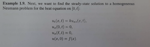
I am going through the literature on Dirichlet and Neumann conditions for the heat equation...i need to be certain on the nonhomogenous bit that is indicated on the excerpt. I am aware that for a pde to be considered homogenous, ##Lu=0## and for it to be non homogenous; ##Lu=f##, where ##L## is the given differential operator.
To determine whether the pde is homogenous or not we make use of the boundary conditions, correct?
In our case we have the given pde with two boundary conditions and one initial condition (not considered due to steady-state condition).
I now get it!
thus to find the solution, we note that since the steady-state is not dependant on time, then it follows that, ##u_{t}=0##
##u(x,t)=u(x)## ##Du_{xx}## =##0→u_{xx}=0## on integration we shall have
##u_{x}=M##, where ##M## is a constant. Integrating again yields
##u(x)=Mx+N##, where ##N## is also a constant. Now using the first boundary conditions, ##u(0,t)=c_1##, we shall have
## c_1=N## on using the second boundary condition, we shall have
##c_2=Ml+c_1## it follows that ##u(x)##=##\dfrac {c_2-c_1}{l}##+##c_1##
cheers guys...
Attachments
Last edited: