Integral limits when using distribution function technique

[lemonthree]

I am not sure about finding the limit of the integral when
it comes to finding the CDF using the distribution function technique.

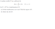
I know that support of y is 0 ≤y<4, and it is
not a one-to-one transformation.

Now, I am confused with part b), finding the limits when calculating the cdf of Y.
Here's my working.
When -1<x<1, it's a two-to-one transformation, 0≤ y<1
P(Y≤y) = P(X^2≤y)
= P(-sqrt(y) ≤ X ≤ sqrt(y) )When -2<x<-1, it's a one-to-one transformation, 1< y<4
P(Y≤y) = P(X^2≤y)
= P(-sqrt(y) ≤ X ≤ sqrt(y) )

The part I'm unsure is in bold. I just can't seem to determine what are the limits...
I've drawn the graph of f(x) against x and y against x, I know it's supposed to help me but I don't know how it relates.

[DESMOS]{"version":7,"graph":{"viewport":{"xmin":-10,"ymin":-12.5,"xmax":10,"ymax":12.5}},"randomSeed":"066490480d2a6d972d994e681ea97f80","expressions":{"list":[{"id":"2","type":"table","columns":[{"values":["-2","-1","0","1",""],"hidden":true,"id":"3","color":"#2d70b3","latex":"x"},{"values":["","","","",""],"id":"4","color":"#c74440","lines":true,"latex":"x^{2}"}]}]}}[/DESMOS]

[DESMOS]{"version":7,"graph":{"viewport":{"xmin":-10,"ymin":-12.5,"xmax":10,"ymax":12.5}},"randomSeed":"febe03824c866a14f1139ed630aebb2e","expressions":{"list":[{"type":"expression","id":"1","color":"#c74440","latex":"f\\left(x\\right)=\\frac{2}{9}\\left(x+2\\right)"},{"id":"2","type":"table","columns":[{"values":["-2","-1","0","1",""],"hidden":true,"id":"3","color":"#2d70b3","latex":"x"},{"values":["","","","",""],"id":"4","color":"#c74440","lines":true,"latex":"f\\left(x\\right)"}]}]}}[/DESMOS]

 

[GJA]

Hi lemonthree,

Everything you've written so far is correct. In particular, noting that there is a difference between $0\leq y \leq 1$ and $1\leq y\leq 4$ is a big key to solving this problem. The very fact that we need to consider two different intervals for $y$ suggests that the CDF will be a piecewise defined function. Consider the case where $0\leq y \leq 1$ (see figure).

[DESMOS]{"version":7,"graph":{"viewport":{"xmin":-3,"ymin":-1,"xmax":3,"ymax":5},"xAxisStep":1,"yAxisStep":1,"squareAxes":false},"randomSeed":"959770bb1c14267b441b441732312797","expressions":{"list":[{"type":"expression","id":"1","color":"#388c46","latex":"y=\\left\\{-2<x<1:\\ x^{2}\\right\\}"},{"type":"expression","id":"2","color":"#000000","latex":"\\left(0,0.75\\right)","showLabel":true,"label":"`{y}`"},{"type":"expression","id":"3","color":"#000000","latex":"y=\\left\\{-\\sqrt{.75}<x<\\sqrt{.75}:\\ 0.75\\right\\}","lineStyle":"DASHED"},{"type":"expression","id":"5","color":"#000000","latex":"\\left(-\\sqrt{.75},0\\right)","showLabel":true,"label":"`-\\sqrt{{y}}`"},{"type":"expression","id":"4","color":"#000000","latex":"\\left(\\sqrt{.75},0\\right)","showLabel":true,"label":"`\\sqrt{{y}}`"},{"id":"9","type":"table","columns":[{"values":["-\\sqrt{.75}","-\\sqrt{.75}"],"hidden":true,"id":"7","color":"#2d70b3","latex":"x_1"},{"values":["0",".75"],"id":"8","color":"#000000","lines":true,"lineStyle":"DASHED","latex":"y_1"}]},{"id":"14","type":"table","columns":[{"values":["\\sqrt{.75}","\\sqrt{.75}"],"hidden":true,"id":"12","color":"#c74440","latex":"x_2"},{"values":[".75","0"],"id":"13","color":"#000000","lines":true,"lineStyle":"DASHED","latex":"y_2"}]}]}}[/DESMOS]

From the diagram above we see that $$P(Y\leq y) = P\left(-\sqrt y\leq X\leq \sqrt y\right).$$ Using the PDF for $X$ the above becomes: $$P(Y\leq y) = \frac{2}{9}\int_{-\sqrt y}^{\sqrt y}(x+2)dx=\frac{8\sqrt y}{9}.$$ Can you see how to do something similar to complete the case where $1\leq y\leq 4$?

 

[lemonthree]

Hi GJA, thank you for the very helpful tips. For 1≤y≤4 , what I did was similar, though not quite the same.
P(Y≤y) = P(X^2≤y)
= P(-2 ≤ X ≤ sqrt(y) )
=$$\int_{-2}^{root(y)} (2/9)(x+2) dx$$
= y/9 + 4/9sqrt(y) + 4/9

Is this correct?

 

[GJA]

Happy to help! You ask great questions and your intuition for mathematical problem solving is quite good.

You're very close to the correct answer and I'd like to see if a few more hints will help you find what needs to be corrected. For the case where $1\leq y\leq 4$ we have the following diagram:

[DESMOS]{"version":7,"graph":{"viewport":{"xmin":-3,"ymin":-1,"xmax":3,"ymax":5},"xAxisStep":1,"squareAxes":false},"randomSeed":"2560b98cc3e1185801770265bac2120a","expressions":{"list":[{"type":"expression","id":"1","color":"#388c46","latex":"y=\\left\\{-2<x<1:\\ x^{2}\\right\\}"},{"type":"expression","id":"2","color":"#c74440","latex":"y\\ =\\ \\left\\{-\\sqrt{2.25}<x<1:\\ 2.25\\right\\}"},{"type":"expression","id":"3","color":"#c74440","latex":"\\left(0,\\ 2.25\\right)","showLabel":true,"label":"`{y}`","dragMode":"NONE"},{"id":"7","type":"table","columns":[{"values":["-\\sqrt{2.25}","-\\sqrt{2.25}"],"hidden":true,"id":"5","color":"#000000","latex":"x_1"},{"values":["0","2.25"],"id":"6","color":"#c74440","lines":true,"lineStyle":"DASHED","latex":"y_1"}]},{"id":"12","type":"table","columns":[{"values":["1","1"],"hidden":true,"id":"10","color":"#6042a6","latex":"x_2"},{"values":["0","2.25"],"id":"11","color":"#c74440","lines":true,"lineStyle":"DASHED","latex":"y_2"}]},{"id":"17","type":"table","columns":[{"values":["-\\sqrt{2.25}","1"],"hidden":true,"id":"15","color":"#388c46","latex":"x_3"},{"values":["0","0"],"id":"16","color":"#c74440","lines":true,"latex":"y_3"}]},{"type":"expression","id":"19","color":"#c74440","latex":"\\left(-\\sqrt{2.25},0\\right)","showLabel":true,"label":"`-\\sqrt{{y}}`"}]}}[/DESMOS]

Take a look at this picture and see if you can figure out what adjustments need to be made to your previous calculation. Note: there are two equally valid ways to do this. Let me know if you're still stuck after giving this a shot.

 

[lemonthree]

The picture is very handy! I'm guessing it should be

P(Y≤y) = P(X^2≤y)
= P(-sqrt(y)≤ X ≤ 1 )

My thoughts for deciding on those values:
For 1≤y≤4, the values of x can range from -2 to 2.
But in this question, x is -2 to 1. Based on the diagram, I need to "fix" the upper limit at 1.
For the lower limit, it would be -sqrt(y) because as both x and y can be -2, there isn't any "limit" restriction.

 

[GJA]

I agree with you 100%; pictures are incredibly helpful when it comes to gaining insight to a problem. As you continue to gain mathematical/statistical experience, you'll learn how to utilize them more and more to your advantage.

The ideas you expressed in your last post are all correct, nicely done! What you've determined is that for $1\leq y\leq 4$, we must compute $$\frac{2}{9}\int_{-\sqrt y}^{1}(x+2)dx.$$ As I mentioned before, there is another way to solve this problem. Since this method is important to be aware of, I'll go through it here.

[DESMOS]{"version":7,"graph":{"viewport":{"xmin":-2.5,"ymin":-0.5,"xmax":1.5,"ymax":4.5},"xAxisStep":1,"yAxisStep":1},"randomSeed":"3110c425eb7a6777826167fc291141b5","expressions":{"list":[{"type":"expression","id":"1","color":"#000000","latex":"y=\\left\\{-2<x<1:\\ x^{2}\\right\\}"},{"type":"expression","id":"2","color":"#c74440","latex":"y=\\left\\{-\\sqrt{2.25}<x<1:\\ 2.25\\right\\}"},{"type":"expression","id":"3","color":"#c74440","latex":"\\left(0,2.25\\right)","showLabel":true,"label":"`{y}`"},{"id":"13","type":"table","columns":[{"values":["-\\sqrt{2.25}","-\\sqrt{2.25}"],"hidden":true,"id":"11","color":"#000000","latex":"x_1"},{"values":["2.25","0"],"id":"12","color":"#c74440","lines":true,"lineStyle":"DASHED","latex":"y_1"}]},{"id":"17","type":"table","columns":[{"values":["1","1"],"hidden":true,"id":"15","color":"#388c46","latex":"x_2"},{"values":["0","2.25"],"id":"16","color":"#c74440","lines":true,"lineStyle":"DASHED","latex":"y_2"}]},{"id":"22","type":"table","columns":[{"values":["-\\sqrt{2.25}","1"],"hidden":true,"id":"20","color":"#2d70b3","latex":"x_3"},{"values":["0","0"],"id":"21","color":"#c74440","lines":true,"latex":"y_3"}]},{"id":"27","type":"table","columns":[{"values":["-2","-\\sqrt{2.25}"],"hidden":true,"id":"25","color":"#c74440","latex":"x_4"},{"values":["0","0"],"id":"26","color":"#2d70b3","lines":true,"latex":"y_4"}]},{"type":"expression","id":"29","color":"#c74440","latex":"\\left(-\\sqrt{2.25},0\\right)","showLabel":true,"label":"`-\\sqrt{{y}}`"}]}}[/DESMOS]

As is hopefully clear from the picture, the interval $-2\leq x\leq 1$ can be broken up into two parts (the blue and the red shown above): $-2\leq x\leq -\sqrt{y}$ and $-\sqrt{y}\leq x\leq 1.$ This is useful because it allows us to write $$P\left(-2\leq x\leq 1\right) = P\left(-2\leq x\leq -\sqrt{y}\right) +P\left(-\sqrt{y}\leq x\leq 1\right).$$ Solving this equation for the the probability corresponding to the red line segment (which is the one we need to know), we get $$P\left(-\sqrt{y}\leq x\leq 1\right) = 1 - P\left(-2\leq x\leq -\sqrt{y}\right).$$ Notice that $P\left(-2\leq x\leq -\sqrt{y}\right)$ is nothing but the CDF for $X$ evaluated at $-\sqrt{y}.$ Hence, $$ P\left(-\sqrt{y}\leq x\leq 1\right) = 1 - F_{X}(-\sqrt{y})=1-\frac{2}{9}\int_{-2}^{-\sqrt{y}}(x+2)dx.$$ I highly encourage you to solve the problem using the method you mentioned in your last post and the one shown here. If done correctly, you will see that the two give the same result.Feel free to let me know if you have any other questions.

 

[lemonthree]

Thank you so much for showing the alternative method, I calculated for both methods and indeed they both gave the same answer of
$$\frac{4\sqrt{y}-y+5}{9}$$

 

[lemonthree]

Oh and I wanted to mention something: I realized that sketching the graph of f(x) in such cases aren't very helpful, compared to sketching the graph of y against x. So when we go about solving similar questions, does it mean that we can "ignore" the graph of f(x), and just sketch y against x? Because all we just need is to chuck f(x) into the integral and solve for it...

 

[GJA]

Thank you so much for showing the alternative method, I calculated for both methods and indeed they both gave the same answer of
$$\frac{4\sqrt{y}-y+5}{9}$$

Nice work! Happy to hear that you were able to see the connection between the two approaches.

To completely finish things off, the CDF for Y is given by $$F_{Y}(y) = \begin{cases}0 & y\leq 0\\
\frac{8\sqrt{y}}{9} & 0\leq y\leq 1\\
\frac{4\sqrt{y}-y+5}{9} & 1\leq y\leq 4\\
1 & y\geq 4 \end{cases}$$

It's worth noting that $\lim_{y\rightarrow 0^{+}}\dfrac{8\sqrt{y}}{9} = 0$ and $\lim_{y\rightarrow 4^{-}}\dfrac{4\sqrt{y}-y+5}{9} = 1,$ as they should because these terms represent the cumulative probability for $Y$ near $y = 0$ and $y=4$, respectively.

 

[GJA]

Oh and I wanted to mention something: I realized that sketching the graph of f(x) in such cases aren't very helpful, compared to sketching the graph of y against x. So when we go about solving similar questions, does it mean that we can "ignore" the graph of f(x), and just sketch y against x? Because all we just need is to chuck f(x) into the integral and solve for it...

I certainly understand what you're going for here and admire your desire to find the most efficient problem solving technique. As a general rule, I would caution against ignoring $f(x)$ completely because it can be used to find the bounds for the graph of $Y$ vs $X$ if they aren't given to you at the beginning. For this problem you were told $-2<x<1$, but it's conceivable you wouldn't be given this in a future exercise. Nevertheless, what you're saying does 100% have merit: Use the graph of $Y$ vs. $X$ to determine what the limits of integration for $f_{X}(x)$ are.

 

[lemonthree]

Alright, I will take note of this, thank you so much for the very helpful tips!