- 4,533
- 13
I'm going to start by asking about an example from class and then hopefully use that to work on the problem I need to solve. Here is an example:
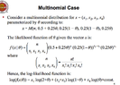
Let's say we have a multinomial distribution $x \sim M(n;.5+.25\theta,0.25(1-\theta),0.25(1-\theta),0.5\theta)$.
The likelihood function of $\theta$ given the vector $x$ is:
$$f(x|\theta) = \frac{n!}{x_1!x_2!x_3!x_4!}(.5+.25\theta)^{x_1}(0.25(1-\theta)^{x_2+x_3}(0.5\theta)^{x_4}$$.
This part is fine. It's this next step that confuses me.
$$\log (f(x|\theta))=x_1 \log(2+ \theta)+(x_2+x_3) \log(1-\theta)+x_4 \log(\theta)+\text{constant}$$
I understand the standard log rules I believe but I don't see how $\log(.5+.25\theta)^{x_1}=x_1 \log(2+ \theta)$. Obviously $x_1$ can be brought down in front of the expression but the stuff inside the parentheses makes no sense.